Introduction and Matrix Multiplication
Software performance engineering was common, because machine resources were limited
- IBM System/360
- Launched: 1964
- Clock rate: 33 KHz
- Data path: 32 bits
- Memory: 534 kbytes
- Cost: $5,000/month
- DEC PDP-11
- Launched: 1970
- Clock rate: 1.25 MHz
- Data path: 16 bits
- Memory: 56 kbytes
- Cost: $2,000/month
- Apple II
- Launched: 1977
- Clock rate: 1 MHz
- Data path: 8 bits
- Memory: 48 kbytes
- Cost: $1,395/month
Programs had to be planned around the machine. Many programs wouldn’t fit without intense performance engineering.
The Moore’s law hit a bottle neck in 2004 where the clock speed can no longer scale. To scale the performace, the vendors started investing on parellel processor aka Multicore. Processor manufactures put many processing cores on the microprocessor chip. Each generation of Moore’s Law potentially doubles number of cores.
A modern multicore desktop processor contains parallel-processing cores, vector units, caches, perfetchters, GPU’s, hyperthreading, dynamic requency scaling, etc. How can we write software to utilize modern hardware efficiently?
Matrix Multiplication
A naive way to do matrix multiplication in python
import sys, random
from time import *

n = 4096
# gernerate float matrices
A = [[random.random() for row in range(n)] for col in range(n)]
B = [[random.random() for row in range(n)] for col in range(n)]
C = [[0 for row in range(n)] for col in range(n)]

start = time()
for i in range(n):
    for j in range(n):
        for k in range(n):
            C[i][j] += A[i][k] * B[k][j]
end = time()
print("%.6f" %(end-start))
Let’s say we have super powerful machine like this.
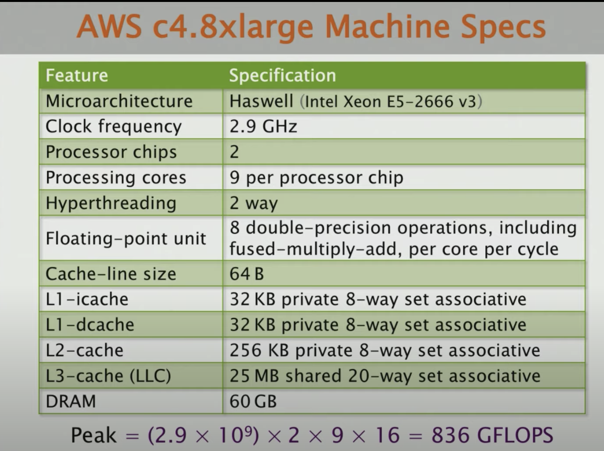
The Python code takes ~6 hours to run on that powerful machine. Let’s break this down.
The algorithm complicity is $2n^3 = 2(2^{12})^3 = 2^{37}$ floating-point-operators. The running time is 21042 seconds. If we divide this two number, we get $2^{37} / 21042 \approx 6.25 (MFLOPS)$ per second. The peak of this machine is around 836 GFLOPS, so Python gets 0.00075% of peak, which is slow.
If we run the same code in Java, it takes 2738 seconds that is about 46 minutes. 8.8x faster than Python. In C, it takes 1156 seconds, 2x faster than Java and about 18x faster than Python.
| version | Implementation | Running time (s) | Relative Speedup | Absolute Speedup | GFLOPS | Percent of peak |
|---|---|---|---|---|---|---|
| 1 | Python | 21042 | 1.00 | 1 | 0.007 | 0.001 |
| 2 | Java | 2738 | 8.81 | 9 | 0.058 | 0.007 |
| 3 | C | 1156 | 2.07 | 18 | 0.119 | 0.014 |
Why is Python so slow and C so fast
- Python is interpreted.
- C is compiled directly to machine code.
- Java is compiled to byte-code, which is then interpreted and JIT compiled to machine code.
- JIT compilers can recover some of the perfomance lost by interpretation
- When code is first executed, it is interpreted
- The runtiem system keeps track of how often the varous pieces of code are exectued
- WHenever some piece of code executes sufficicently frequently, it gets compiled to machine code in real time.
- Future executions of that code use the more-efficent compiled version
Loop Order
Another optimization approach is to change the order of the loop. Changing the order of i,j,k doesn’t affect the correctness of the algorithm, but can give a huge perf boost
| version | Implementation | Running time (s) | Relative Speedup | Absolute Speedup | GFLOPS | Percent of peak |
|---|---|---|---|---|---|---|
| 1 | Python | 21042 | 1.00 | 1 | 0.007 | 0.001 |
| 2 | Java | 2738 | 8.81 | 9 | 0.058 | 0.007 |
| 3 | C | 1156 | 2.07 | 18 | 0.119 | 0.014 |
| 4 | Interchange loops | 177.68 | 6.5 | 118 | 0.774 | 0.093 |
It turns out by just simply changing the order of the loop, the running time is affected by a factor of 18. So what’s going on?
Each processor reads and writes main memory in contiguous block, caclled cache lines.
- Previously accessed cache lines are stored in a smaller memory, called cache, that sits near the processor
- Cache hits - access to data in cache
- Cache misses - access to data not in cache
So the general rule is to avoid the cache misses. Once we load a piece of memory into cache, we want to reuse it as much as possible. Now let’s see how we load matrices into memroy.
The matrices are laid out in memory in row-major order. What does this layout imply about the performance of different loop orders? Let’s take a look at the original loop order
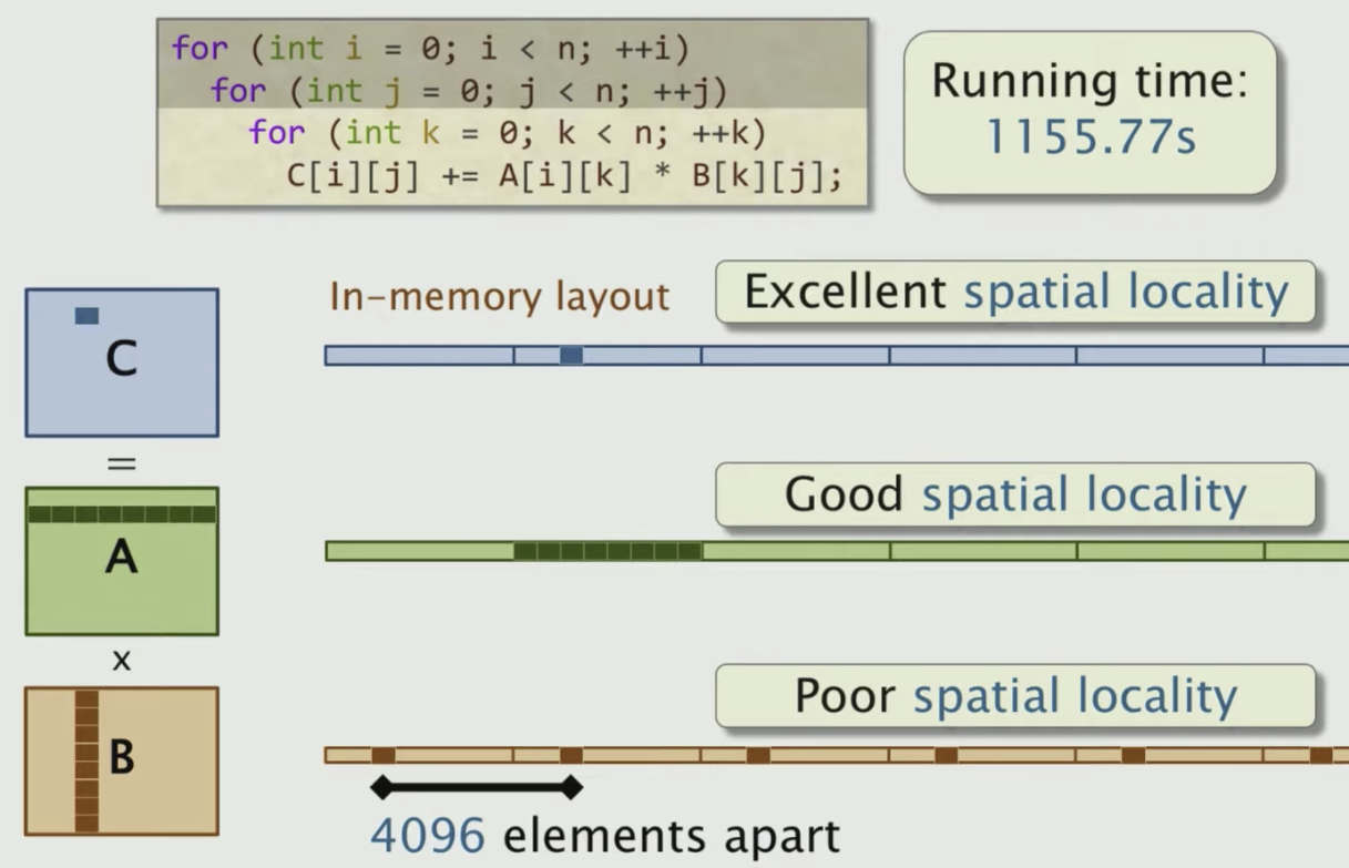
As we can see in pic, for C, since we keep updating it, it gets really nice spatial locality (stays in the cache). For A, we go through a linear order, we get a good spatial locality due to the contiguous access. But for B, the access of a each element is distributed far away in memory, not in contiguous postions. So it’s not good for caching.
Let’s take a look at different other ones as shown below
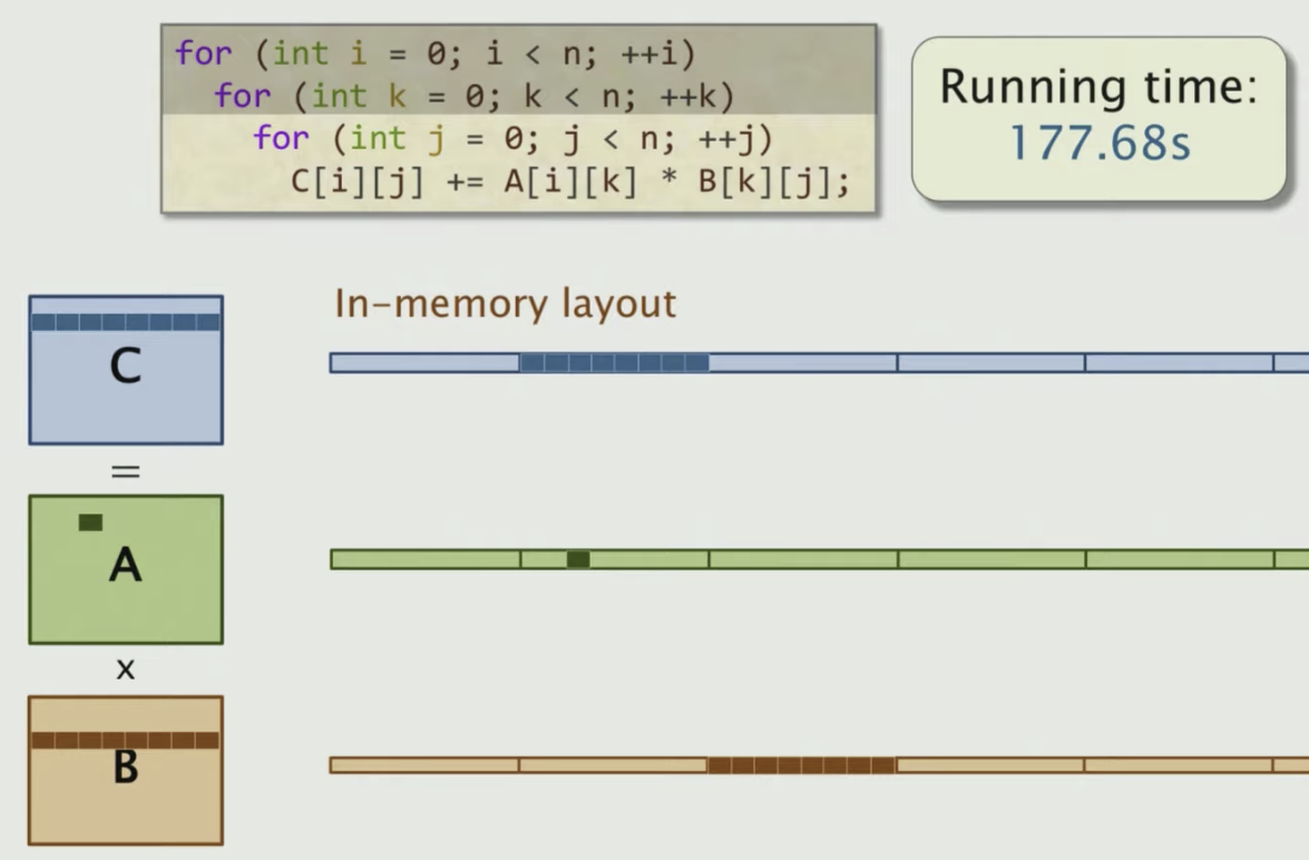

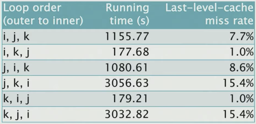
We can just measure the effect of different accesss patterns using the Cachegrind cache simulator
$ valgrind --tool=cachegrind ./mm
Compiler Optimizations
Clang provides a collection of optimization switches. You can specify a switch to the compiler to ask it to optimize.
| Opt. level | Meaning | Time (s) |
|---|---|---|
| -O0 | Do not optimize | 177.54 |
| -O1 | Optimize | 66.24 |
| -O2 | Optimize even more | 54.63 |
| -O3 | Optimize yet more | 55.58 |
Clang also supports opitmization levels for special purpose, such as -Os, which aims to limit code size, and -Og, for debugging purposes.
With this simple code and compiler technology, we can achieve 0.3% of the peak performance of the machine.
| version | Implementation | Running time (s) | Relative Speedup | Absolute Speedup | GFLOPS | Percent of peak |
|---|---|---|---|---|---|---|
| 1 | Python | 21042 | 1.00 | 1 | 0.007 | 0.001 |
| 2 | Java | 2738 | 8.81 | 9 | 0.058 | 0.007 |
| 3 | C | 1156 | 2.07 | 18 | 0.119 | 0.014 |
| 4 | + Interchange loops | 177.68 | 6.5 | 118 | 0.774 | 0.093 |
| 5 | + compiler falgs | 54.64 | 3.25 | 385 | 2.526 | 0.301 |
Multicore parallelism
The cilk_for loop allows all iterations of the loop to execute in parallel.
cilk_for(int i=0; i<n; ++i){
    for(int k=0; k<n; ++k) {
        for(int j=0; j<n; ++j) {
            C[i][j] += A[i][k] * B[k][j]
        }
    }
}
Here we paralle the i loop, which leads to 3.18s. But we can also parallelize the inner loops, such as j loop and k loop.
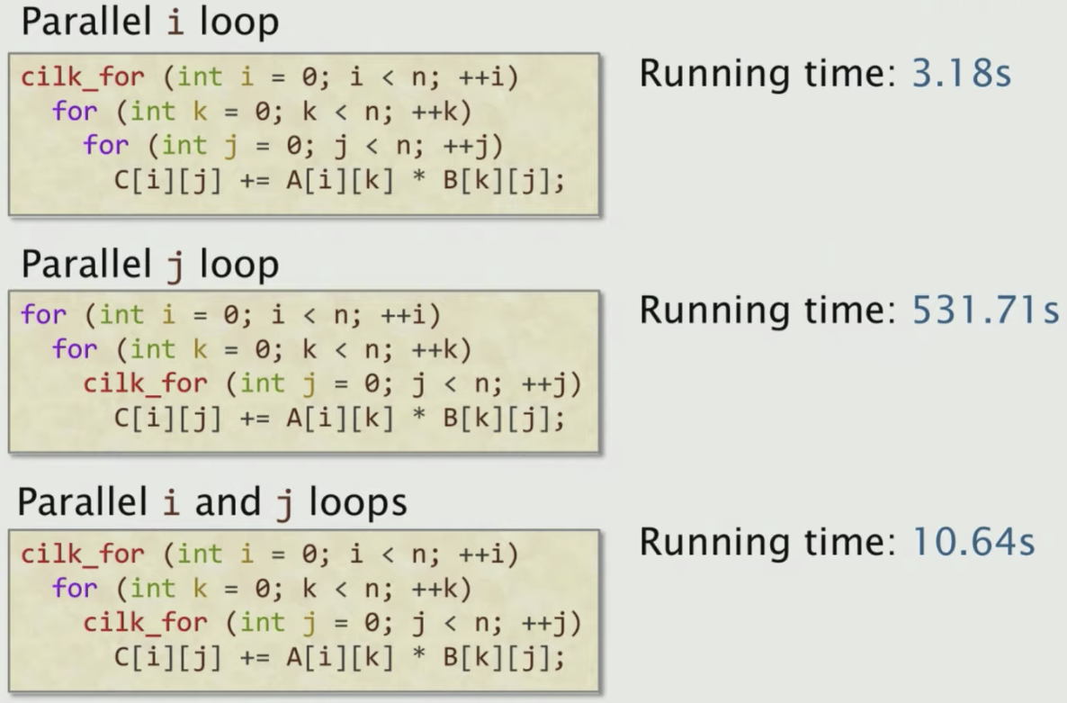
It turns out the scheduling overhead for parallelizing inner loops will out-weighted the benifit, so it becomes slower than just parallelizing the outer loop. So the “Rule of Thumb” here is always parallelize outer loop rather than inner loops.
| version | Implementation | Running time (s) | Relative Speedup | Absolute Speedup | GFLOPS | Percent of peak |
|---|---|---|---|---|---|---|
| 1 | Python | 21042 | 1.00 | 1 | 0.007 | 0.001 |
| 2 | Java | 2738 | 8.81 | 9 | 0.058 | 0.007 |
| 3 | C | 1156 | 2.07 | 18 | 0.119 | 0.014 |
| 4 | + Interchange loops | 177.68 | 6.5 | 118 | 0.774 | 0.093 |
| 5 | + compiler falgs | 54.64 | 3.25 | 385 | 2.526 | 0.301 |
| 6 | Parallel loops | 3.04 | 17.97 | 6921 | 45.211 | 5.408 |
Using parallel loops gets us almost 18x speedup on 18 cores (Disclaimer: Not all code is so easy to parallelize effectively).
Hardware Caches, Revisited
IDEA: Restructure the computation to reuse data in the cache as much as possible.
- Cache misses are slow, and cache hits are fast.
- Try to make the most of the cache by reusing the data that’s already there.
How many memory accesses must the looping code perform to fully compute 1 row of C?
4096 * 1 = 4096writes toC4096 * 1 = 4096reads toA4096 * 4096 = 16,777,216reads fromB
That is 16,785,408 memory access in total for just computing a row of C as shown below

What if we compute blocks rather than rows in matrics? Would that be faster?
Say we divide C into multiple blocks. For each block, it is 64x64. To compute each block we need
64 * 64 = 4096writes toC64 * 4096 = 262,144reads from A4096 * 64 = 262,144reads fromB
That is 528,384 memory accesses in total.

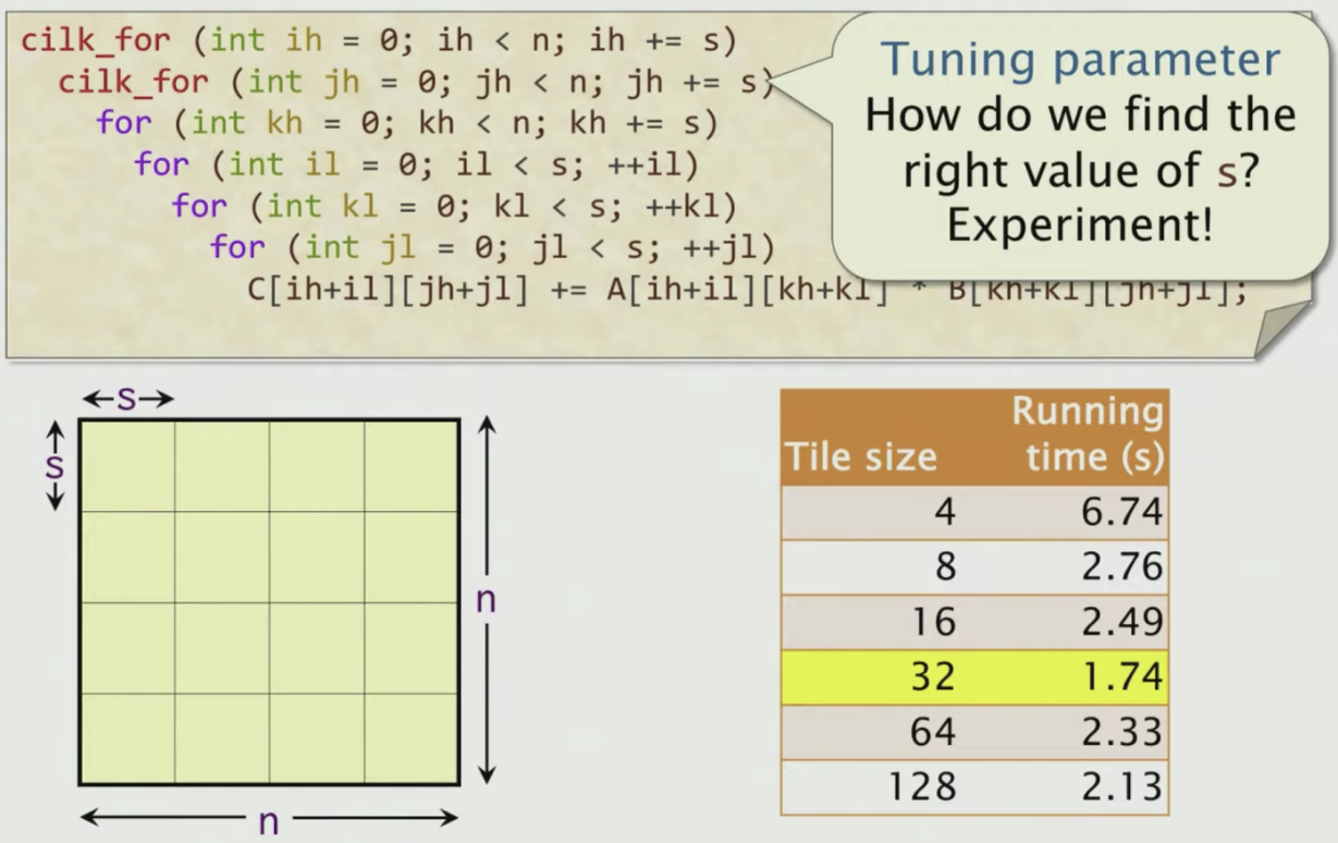
To implement that, we turn the code above to a tiled Matrix Multiplication
cilk_for(int ih=0; ih<n; ih += s) {
    cilk_for(int jh=0; jh<n; jh += s) {
        for(int kh=0; kh<n; kh += s) {
            for(int il=0; il<s; ++il) {
                for(int kl=0; kl<s; ++kl) {
                    for(int jl=0; jl<s; ++jl) {
                        C[ih+il][jh+jl] += A[ih+il][kh+kl] * B[kh+kl][jh+jl];
                    }
                }
            }
        }
    }
}
s is a tuning parameter to control how big is the tile. In this case, 32 is the best number.
| version | Implementation | Running time (s) | Relative Speedup | Absolute Speedup | GFLOPS | Percent of peak |
|---|---|---|---|---|---|---|
| 1 | Python | 21042 | 1.00 | 1 | 0.007 | 0.001 |
| 2 | Java | 2738 | 8.81 | 9 | 0.058 | 0.007 |
| 3 | C | 1156 | 2.07 | 18 | 0.119 | 0.014 |
| 4 | + Interchange loops | 177.68 | 6.5 | 118 | 0.774 | 0.093 |
| 5 | + compiler falgs | 54.64 | 3.25 | 385 | 2.526 | 0.301 |
| 6 | Parallel loops | 3.04 | 17.97 | 6921 | 45.211 | 5.408 |
| 7 | +tiling | 1.79 | 1.70 | 11,772 | 76.782 | 9.184 |
The tiled implementation performs about 62% fewer cache references and incurs 68% fewer cache misses.
It turns out with the L3 caches, we can do nested tiled loops (a bit compilicated, not going to explain in detail.)
| version | Implementation | Running time (s) | Relative Speedup | Absolute Speedup | GFLOPS | Percent of peak |
|---|---|---|---|---|---|---|
| 1 | Python | 21042 | 1.00 | 1 | 0.007 | 0.001 |
| 2 | Java | 2738 | 8.81 | 9 | 0.058 | 0.007 |
| 3 | C | 1156 | 2.07 | 18 | 0.119 | 0.014 |
| 4 | + Interchange loops | 177.68 | 6.5 | 118 | 0.774 | 0.093 |
| 5 | + compiler falgs | 54.64 | 3.25 | 385 | 2.526 | 0.301 |
| 6 | Parallel loops | 3.04 | 17.97 | 6921 | 45.211 | 5.408 |
| 7 | +tiling | 1.79 | 1.70 | 11,772 | 76.782 | 9.184 |
| 8 | Parallel divide-and-conquer | 1.30 | 1.38 | 16,197 | 105.722 | 12.646 |
Vectorization
Modern microprocessors incorporate vector hardware to process data in a Single-Instruction stream, Multiple-Data stream (SIMD) fashion.
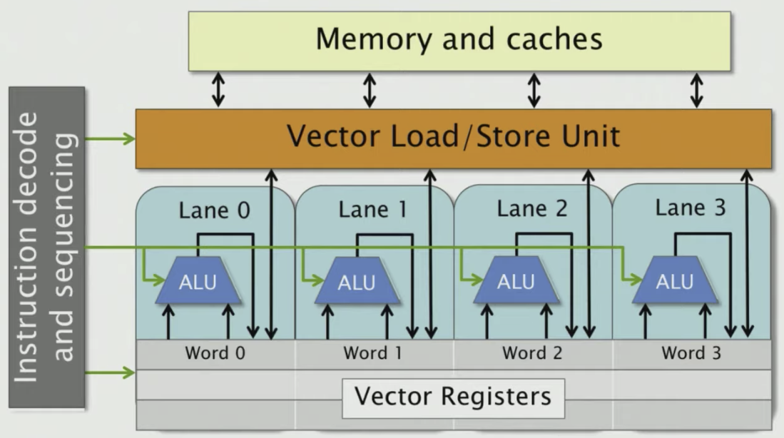
Each vector register holds multiple words of data so CPU can load multiple bytes in one instruction. In the pic above, let’s say 1 word = 32 bits and vector register can hold 4 words which are 128 bits (16 bytes). We know a float number is 4 bytes, then one SIMD instruction can load 4 float numbers.
Clang/LLVM uses vector instructions automatically when compiling at optimization level -O2 or higher. Clang/LLVM can be induced to produce a vectorization report as follows:
$ clang -03 -std=c99 mm.c -o mm -Rpass=vector
The command tells you which part of your code will be vectorized. Many machines don’t support the newest set of vector instructions, however, so the compiler uses vector instructions conservatively by default. Programmers can direct the compiler to use modern vector instructions using compiler flags such as the following:
-mavx: Use Intel AVX vector instructions.-mavx2: Use Intel AVX2 vector instructions.-mfma: Use fused multiply-add vector instructions.-march=<string>: Use whatever instructions are available on the specific arch.
Due to restrictions on floating-point arithmetic, additional flags, such as -ffast-math migth be needed for these vectorization flags to have an effect.
Using the flag -march=native and -ffast-math nearly doubles the performance.
| version | Implementation | Running time (s) | Relative Speedup | Absolute Speedup | GFLOPS | Percent of peak |
|---|---|---|---|---|---|---|
| 1 | Python | 21042 | 1.00 | 1 | 0.007 | 0.001 |
| 2 | Java | 2738 | 8.81 | 9 | 0.058 | 0.007 |
| 3 | C | 1156 | 2.07 | 18 | 0.119 | 0.014 |
| 4 | + Interchange loops | 177.68 | 6.5 | 118 | 0.774 | 0.093 |
| 5 | + compiler falgs | 54.64 | 3.25 | 385 | 2.526 | 0.301 |
| 6 | Parallel loops | 3.04 | 17.97 | 6921 | 45.211 | 5.408 |
| 7 | +tiling | 1.79 | 1.70 | 11,772 | 76.782 | 9.184 |
| 8 | Parallel divide-and-conquer | 1.30 | 1.38 | 16,197 | 105.722 | 12.646 |
| 9 | + compiler vectorization | 0.7 | 1.87 | 30.272 | 196.341 | 23.468 |
AVX Intrinsic Instructions
Instead of letting compiler vectorize your code, you can also use the AVX instructions directly. Intel provies C-style functions, called instrinic instructions, that provide direct access to hardware vector operations.
| version | Implementation | Running time (s) | Relative Speedup | Absolute Speedup | GFLOPS | Percent of peak |
|---|---|---|---|---|---|---|
| 1 | Python | 21042 | 1.00 | 1 | 0.007 | 0.001 |
| 2 | Java | 2738 | 8.81 | 9 | 0.058 | 0.007 |
| 3 | C | 1156 | 2.07 | 18 | 0.119 | 0.014 |
| 4 | + Interchange loops | 177.68 | 6.5 | 118 | 0.774 | 0.093 |
| 5 | + compiler falgs | 54.64 | 3.25 | 385 | 2.526 | 0.301 |
| 6 | Parallel loops | 3.04 | 17.97 | 6921 | 45.211 | 5.408 |
| 7 | +tiling | 1.79 | 1.70 | 11,772 | 76.782 | 9.184 |
| 8 | Parallel divide-and-conquer | 1.30 | 1.38 | 16,197 | 105.722 | 12.646 |
| 9 | + compiler vectorization | 0.7 | 1.87 | 30,272 | 196.341 | 23.468 |
| 10 | + AVX instrinsics | 0.39 | 1.76 | 53,292 | 352.408 | 41.677 |
We stop here as it beats the Intel MKL library which contains engineered math kernels for doing matmul (only for the 4096 x 4096 case).
