线性回归

Posted on 2017-08-20 | In Machine Learning , AI

回归问题

回归分析(Regression Analysis)是一种统计学上分析数据的方法，目的在于了解两个或多个变数间是否相关、相关方向与强度，并建立数学模型以便观察特定变数来预测研究者感兴趣的变数。更具体的来说，回归分析可以帮助人们了解在只有一个自变量变化时因变量的变化量，因此可以用来做数据预测。

一维线性回归

假设我们获得了一份房子大小和价格数据集，如下表所示

Size(x)	Price(y)
2104	460
1035	224
868	230
642	126
…	…

我们的任务是找到房价和房屋大小的关系函数，使我们可以根据房子大小来预测房价。显然，我们可以设计一个简单的一维线性函数

h_{θ} (x) = θ_{0} + θ_{1} x

其中 $x$ 表示房屋大小， $h_{θ} (x)$ 表示我们的预测结果。在这个函数中 $θ_{0}$ 和 $θ_{1}$ 是未知的，我们怎么评价这个预测函数的效果呢？显然我们需要将预测结果 $h_{θ} (x) =$ 和真实结果 $y$ 进行比对，比对的方法有 $| h_{θ} (x) - y |$ 或者 $(h_{θ} (x) - y)^{2}$ ，只要这个值越小，我们就认为我们的预测函数的误差最小，于是我们需要引入一个Cost函数

代价函数

J (θ_{0}, θ_{1}) = \frac{1}{2 m} \sum_{i = 1}^{m} ({\hat{y}}_{i} - y_{i})^{2} = \frac{1}{2 m} \sum_{i = 1}^{m} (h_{θ} (x_{i}) - y_{i})^{2}

这个式子的含义是找到 $θ_{0}$ 和 $θ_{1}$ 的值使 $J (θ_{0}, θ_{1})$ 的值最小，其中 $m$ 为训练样本 $x$ 的个数，为了求导方便系数乘了1/2。可见 $J (θ_{0}, θ_{1})$ 是一个二元函数。

二维梯度下降

由于我们的 $J (θ_{0}, θ_{1})$ 是一个convex函数，因此它存在极小值点，为了找到 $θ_{0}$ , $θ_{1}$ 使 $J (θ_{0}, θ_{1})$ 值最小，我们需要不断改变他们的值，直到找到 $θ_{0}$ ,和 $θ_{1}$ ，使 $J (θ_{0}, θ_{1})$ 在改点处的导数为0。

那么 $θ_{0}$ ,和 $θ_{1}$ 该如何快速的变化到我们想找的点呢？这里就要使用梯度下降法

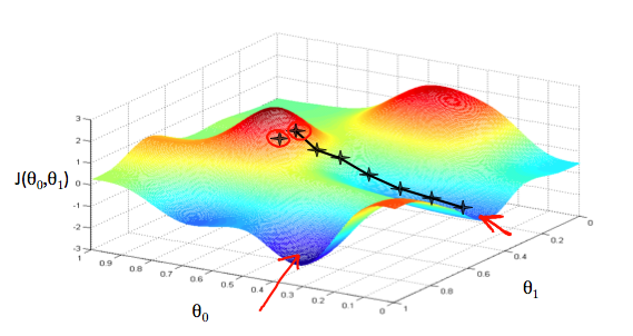
θ_{j} := θ_{j} - α \frac{\partial J (θ_{0}, θ_{1})}{\partial θ_{j}}

梯度下降是求多维函数的极值方法，因此上述公式是对 $θ_{j}$ 求导，每一个 $θ_{j}$ 代表一元参数，也可以理解为一维向量，上述 case 中，只有 $θ_{0}$ 和 $θ_{1}$ 两个参数，可以理解在这两个方向上各自下降，下降过程是一个不断迭代的过程，直到 $θ_{j}$ 收敛停止变化。如下图所示

对上述例子，我们只需要分别对 $θ_{0}$ ,和 $θ_{1}$ 进行梯度下降，直至它们收敛

\begin{aligned} θ_{0} & := θ_{0} - α \frac{1}{m} \sum_{i = 1}^{m} (h_{θ} (x_{i}) - y_{i}) \\ θ_{1} & := θ_{1} - α \frac{1}{m} \sum_{i = 1}^{m} (h_{θ} (x_{i}) - y_{i}) \cdot x_{i} \end{aligned}

注意，上述例子中我们的cost函数是凸函数(convex function)，因此上述两个式子没有局部极值点，只有全局唯一的一个极值点。梯度下降法通常在离极值点远的地方下降很快，但在极值点附近时会收敛速度很慢。因此，梯度下降法的解是全局最优解。而在一般情况下，梯度下降法不保证求得全局最优解。

多维线性回归

回到第一节开头的例子，实际生活中影响房价的因素很多，比如房屋数量，楼层数等等，因此房价的变化是多个变量相互作用的

Size(x1)	#bed room (x2)	#floors(x3)	Price(y)
2104	5	2	460
1035	4	1	224
868	3	2	230
642	2	1	126
…	…	…	…

由于多个feature的影响，此时我们的预测函数将变成多维：

h_{θ} (x) = \sum_{j = 0}^{n} θ_{j} x_{j} = θ_{0} + θ_{1} x_{1} + + θ_{2} x_{2} + . . . + θ_{n} x_{n}

注意上述式子中 $x_{0}$ 默认为1，即 $x_{0}^{(i)} = 1$

如果将 $x$ 和 $θ$ 式子用向量表示，则上述式子也可以表示为：

h_{θ} (x) = [\begin{matrix} θ_{0} & θ_{1} & . . . & θ_{n} \end{matrix}] [\begin{matrix} x_{0} \\ x_{1} \\ . . . \\ x_{n} \end{matrix}] = θ^{T} x

上述式子给出了单个样本的预测函数，实际应用中上我们的数据集里有多个样本，这里我们用上角标表示，如下

$m$ 表示样本数
$n$ 表示feature个数
$x^{(i)}$ 表示第 $i$ 组训练样本
$x_{j}^{(i)}$ 表示第 $i$ 个样本中的第 $j$ 个feature

注意，前面一维线性归回的预测函数中，每条样本用 $(x_{i}, y_{i})$ 表示，原因是我们只有一个feature，我们可以用下角标表示每条数据，后面我们统一使用上角标来表示

举例来说， $x^{(2)}$ 表示第二组训练集：

x^{(2)} = [\begin{matrix} 1035 & 4 & 1 & 224 \end{matrix}]

多维梯度下降

参考前面二维梯度下降的求法，多维梯度下降的求法相同

\begin{aligned} θ_{0} & := θ_{0} - α \frac{1}{m} \sum_{i = 1}^{m} (h_{θ} (x_{0}^{(i)}) - y^{(i)}) \cdot x_{0}^{(i)} \\ θ_{1} & := θ_{1} - α \frac{1}{m} \sum_{i = 1}^{m} (h_{θ} (x_{1}^{(i)}) - y^{(i)}) \cdot x_{1}^{(i)} \\ θ_{2} & := θ_{2} - α \frac{1}{m} \sum_{i = 1}^{m} (h_{θ} (x_{2}^{(i)}) - y^{(i)}) \cdot x_{2}^{(i)} \\ ⋮ \\ θ_{n} & := θ_{n} - α \frac{1}{m} \sum_{i = 1}^{m} (h_{θ} (x_{n}^{(i)}) - y^{(i)}) \cdot x_{n}^{(i)} \end{aligned}

线性回归梯度计算的 Ocatave Demo

function [theta, J_history] = gradientDescentMulti(X, y, theta, alpha, num_iters)
%GRADIENTDESCENTMULTI Performs gradient descent to learn theta
%   theta = GRADIENTDESCENTMULTI(x, y, theta, alpha, num_iters) updates theta by
%   taking num_iters gradient steps with learning rate alpha

% Initialize some useful values
m = length(y); % number of training examples
J_history = zeros(num_iters, 1);

for iter = 1:num_iters

    num_features = size(X,2);
    h = X*theta;

    for j = 1:num_features
        x = X(:,j);
        theta(j) = theta(j) - alpha*(1/m)*sum((h-y).* x);
    end

    % ============================================================

    % Save the cost J in every iteration
    J_history(iter) = computeCostMulti(X, y, theta);

end

end

Feature Scaling

Idea: Make sure features are on a similar scale, e.g.,

x1 = size(0-200 feet)
x2=number of bedrooms(1-5)

这种情况 contour 图是一个瘦长的椭圆, 在不优化的情况下，这类梯度下降速度很慢。如果我们将x1和x2做如下调整：

x1 = size(0-200 feet)/5
x2=(number of bedrooms)/5

则 contour 图会变为接近圆形，梯度下降收敛的速度会加快。通常为了加速收敛，会将每个 feature 值(每个xi)统一到某个区间里，比如

0 \leq x_{1} \leq 3, - 2 \leq x_{2} \leq 0.5

Mean normalization

Replace $x_{i}$ with $x_{i} - μ_{i}$ to make features have approximately zero mean.

实际上就是将 feature 归一化，例如

x1=(size-1000)/2000
x2=(#bedrooms-2)/5

则有 $- 0.5 \leq x_{1} \leq 0.5, - 0.5 \leq x_{2} \leq 0.5$

$μ_{i}$ 是所有 $x_{i}$
$μ_{i}$ 是 x_i 的区间范围，即 $(max - min)$

Note that dividing by the range, or dividing by the standard deviation, give different results. For example, if $x_{i}$ represents housing prices with a range of 100 to 2000 and a mean value of 1000, then

x_{i} := \frac{price - 1000}{1900}

μ表示所有 feature 的平均值
s = max - min

Learning Rate

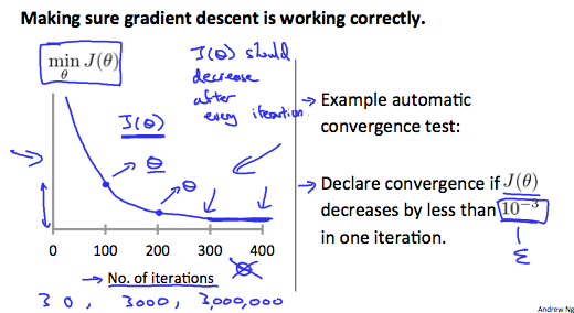
θ_{j} := θ_{j} - α \frac{\partial J (θ)}{\partial θ_{j}}

这节讨论如何选取α。为了求解J(θ)的最小值，梯度下降会不断的迭代找出最小值，理论上来说随着迭代次数的增加，J(θ)将逐渐减小，如图：

Altext

但是如果α选取过大，则可能会导致越过极值点的情况，导致随着迭代次数的增加，J(θ)的值增加或忽高忽低不稳定的情况:

Altext

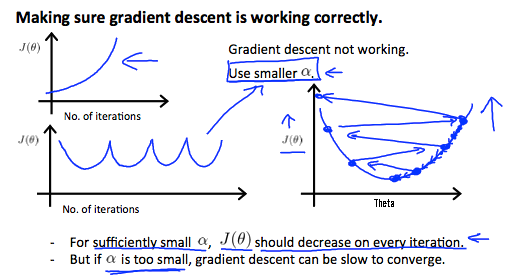
解决办法都是选取较小的α值

if α is too small -> slow convergence
if α is too large -> J(θ)may not decrease on every iteration; may not converge
To choose α , try: …, 0.001, 0.003, 0.01,0.03, 0.1,0.3, 1, …

Polynomial regression

对于线性回归函数:

h_{θ} (x) = θ_{0} + θ_{1} x_{1} + θ_{2} x_{2} + θ_{3} x_{3} + \dots + θ_{n} x_{n}

其中 $x_{i}$ 代表 feature 种类，有些情况下使用这些 feature 制作目标函数不方便，因此可以考虑重新定义 feature 的值。

We can improve our features and the form of our hypothesis function in a couple different ways. We can combine multiple features into one. For example, we can combine x1 and x2 into a new feature x3 by taking x1⋅x2.

例如我们可以将两个 feature 合成一个:x3 = x1*x2，使用x3作为先行回归的 feature 值。

另外，如果只有一个 feature，而使用线性函数又不适合描述完整的数据集，可以考虑多项式函数，比如使用二次函数或者三次函数：

h_{θ} (x) = θ_{0} + θ_{1} x_{1} + θ_{2} x_{1}^{2}

or

h_{θ} (x) = θ_{0} + θ_{1} x_{1} + θ_{2} x_{1}^{2} + θ_{3} x_{1}^{3}

可以令 $x_{2} = x_{1}^{2}, x_{3} = x_{1}^{3}$ ，但是这么选择的一个问题在于 feature scaling 会比较重要，如果 $x_{1}$ 的 range 是 $[1, 1000]$ ，那么 $x_{2}$ 的 range 就会变成 $[1, 1000000]$ 等。

Normal Equation

对于 cost 函数：

J (θ) = \frac{1}{2 m} \sum_{i = 1}^{m} {(h_{θ} (x_{i}) - y_{i})}^{2}

前面提到的求 J(θ) 最小值的思路是使用梯度下降法，对 $θ_{j}$ 求偏导得到各个 θ 值:

\frac{\partial J (θ)}{\partial θ_{j}} = 0 (for every j)

出了梯度下降法之外，还有一种方法叫做Normal Equation，这种方式不需要迭代，可以直接计算出θ值

假设我们有 $m$ 个样本。特征向量的维度为 $n$ 。因此，可知样本为

${(x^{(1)}, y^{(1)}), (x^{(2)}, y^{(2)}), \dots, (x^{(m)}, y^{(m)})}$ 其中对于每一个样本中的 $x^{(i)}$ ，都有 $x^{(i)} = {x_{1}^{(i)}, x_{2}^{(i)}, \dots, x_{n}^{(i)}}$

令线性回归函数：

h_{θ} (x) = θ_{0} + θ_{1} x_{1} + θ_{2} x_{2} + θ_{3} x_{3} + \dots + θ_{n} x_{n}

则有：

X = [\begin{matrix} 1 & x_{1}^{(1)} & x_{2}^{(1)} & \dots & x_{n}^{(1)} \\ 1 & x_{1}^{(2)} & x_{2}^{(2)} & \dots & x_{n}^{(2)} \\ 1 & \dots & \dots & \dots & \dots \\ 1 & x_{1}^{(m)} & x_{2}^{(m)} & \dots & x_{n}^{(m)} \end{matrix}] θ = [\begin{matrix} θ_{1} \\ θ_{2} \\ ⋮ \\ θ_{n} \end{matrix}] Y = [\begin{matrix} y_{1} \\ y_{2} \\ ⋮ \\ y_{m} \end{matrix}]

$X$ 是 $m \times (n + 1)$ 的矩阵
$θ$ 是 $(n + 1) \times 1$ 的矩阵
$Y$ 是 $m \times 1$ 的矩阵

看个例子：

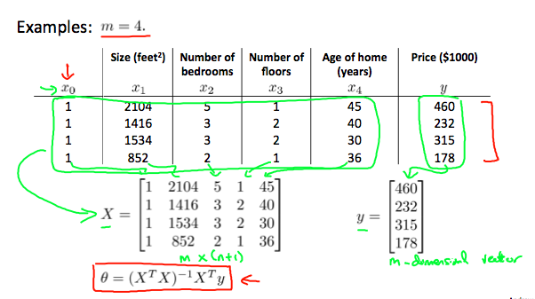
若希望 $h_{(θ)} = y$ ，则有 $X \cdot θ = Y$ ，回想 单位矩阵 和 矩阵的逆 的性质：

单位矩阵 $E$ ， $A E = E A = A$
矩阵的逆 $A^{- 1}$ ， $A$ 必须为方阵， $A A^{- 1} = A^{- 1} A = E$

再来看看式子 $X \cdot θ = Y$ ，若想求出 $θ$ ，那么我们需要做一些转换：

先把 $θ$ 左边的矩阵变成一个方阵。通过乘以 $X^{T}$ 可以实现，则有：
$X^{T} X \cdot θ = X^{T} Y$
把 $θ$ 左边的部分变成一个单位矩阵，这样左边就只剩下 $θ$ ：
$(X^{T} X)^{- 1} X^{T} X \cdot θ = (X^{T} X)^{- 1} X^{T} Y$
由于 $(X^{T} X)^{- 1} X^{T} X = E$ ，因此式子变为：

$θ = (X^{T} X)^{- 1} X^{T} Y$ 这就是 Normal Equation 的表达式。

如果用 Octave 表示，命令为：pinv(X'*X)*X'*Y

什么 case 适合使用 Normal Equation，什么 case 适合使用 Gradient Descent？

Gradient Descent	Normal Equation
Need to choose alpha	No need to choose alpha
Needs many iterations	No need to iterate
$O (k n^{2})$	$O (n^{3})$ need to calculate inverse of $X^{T} X$
Works well when n is large	Slow if n is very large

当样本数量 $n \geq 1000$ 时，使用梯度下降，小于这个数量时，使用 Normal Equation 更方便。当 $n$ 太大时，计算 $X^{T} X$ 会非常慢。

When implementing the normal equation in Octave, we want to use the pinv function rather than inv. The pinv function will give you a value of $θ$ even if $X^{T} X$ is not invertible (不可逆).

If $X^{T} X$ is noninvertible, the common causes might be:

Redundant features, where two features are very closely related (i.e. they are linearly dependent)
Too many features (e.g. m ≤ n). In this case, delete some features or use “regularization” (to be explained in a later lesson).

Solutions to the above problems include deleting a feature that is linearly dependent with another or deleting one or more features when there are too many features.