逻辑回归

Posted on 2017-09-27 | In Machine Learning , AI

文中所用到的图片部分截取自Andrew Ng在Cousera上的课程

逻辑回归

上一节的线性回归可以看到，回归问题在数学上来说是建立$y$与$x$之间关系的模型，给定一个点集，能够用一条曲线去拟合之，如果这个曲线是一条直线，那就被称为线性回归，如果曲线是一条二次曲线，就被称为二次回归，回归还有很多的变种，等等。如果得到的预测函数得出的结果是离散的，我们把这种学习问题叫做分类问题。逻辑回归经常用于解决分类问题, 比如Email是否为Spam/非Spam, 肿瘤是否为恶性/良性，可用下面式子表达

\[y ∈ {0,1}\]

对于分类场景，使用线性回归模型不适合，原因是 $h_{\theta}(x)$ 值不能保证只有0或1，因此我们需要对线性模型做一些改进。

Sigmoid函数

在给出模型前，我们先假设$y$的取值是连续的，则对于任意的输入有

\[0≤h_{\theta}(x)≤1\]

为了达到这个目的，我们需要一个非线性函数$g(x)$将$h_{\theta}(x)$的输出映射到0和1之间，即$h_{\theta}(x)=\theta^{T}x$ 做如下变换：$h_{\theta}(x)=g(\theta^{T}x)$, 其中$g$为

\[g(z)=\frac{1}{1+e^{-z}}\]

可以得到$g(x)$的函数曲线如下

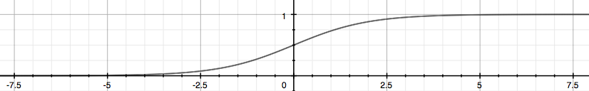
我们看到函数$g(x)$ 将所有实数映射到了(0,1]空间内, 则$g(z)$ 也叫做Sigmoid Function。

Linear Decision Boundary

通过观察函数曲线可以发现，当z大于 0 的时候g(z)≥0.5，因此只需要判断$\theta^{(T)}x$和0的关系即可：

$\theta^{(T)}x ≥ 0$ 可推出 $y=1$
$\theta^{(T)}x < 0$ 可推出 $y=0$

举个例子，假设有一个二维线性预测函数为

\[h_{\theta}(x) = g(\theta_0 + \theta_1x_1 + \theta_2x_2)\]

现在假设θ值已确定为[-3,1,1]，则问题变为求如果要y=1，那么需要 $h(x) = -3 + x_1+x_2 ≥ 0$, 即找到$x_1$, $x_2$满足 $x_1 + x_2 ≥ 3$，如下图所示：

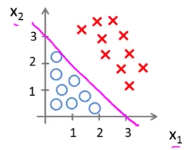
由上图可看出, 图中的粉色线段为可以作为Decision Boundary。当$x_1 + x_2 ≥ 3$时预测结果$y=1$，反之，当$x_1 + x_2 < 3$时，预测结果$y=0$

Non-linear Decision Boundary

接下来我们看一个非线性的预测函数，例如：

\[h_{\theta}x = g(\theta_0 + \theta_1x_1 + \theta_2x_2 + \theta_3x_1{^2} + \theta_4x_2{^2})\]

假设θ值已经确定为[-1,0,0,1,1]，同上，变为求如果要y=1，那么需要$-1 + x_1{^2} + x_2{^2} ≥ 0$，即找到$x_1$, $x_2$满足$x_1^2 + x_2^2 ≥ 0$，则边界函数为$x_1^2 + x_2^2 = 0$，如下图所示

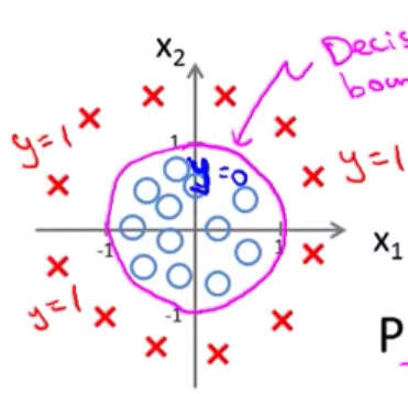
处于粉色圆圈内的样本点预测结果为0, 对于落在圈外的样本点，则预测结果为1。因此这种边界称为非线性的Decision Boundary

Cost Function

可以看到，所谓的逻辑回归，就是通过sigmoid函数将某个预测函数（可能是非线性函数）的值域限定在某个区域内，从而达到对输出进行分类的效果。因此当我们有了模型以后，接下来的问题便是找到一个代价函数来求解θ值，如果使用之前现行回归的 cost function，即

\[J(\theta) =\frac{1}{2m}\sum_{i=1}^m(h_\theta(x_i)-y_i)^2\]

由于$h(x)$变成了复杂的非线性函数，这时会出现$J(\theta)$存才多个local minimum的情况，即$J(\theta)$不是一个convex function，因此梯度下降无法得到最小值。因此我们要找到一个新的代价函数

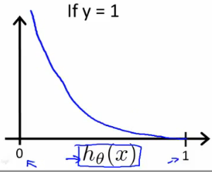
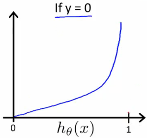
\[Cost(h_\theta(x),y) =\begin{cases}-log(h_\theta(x)), & \text{if $y=1$} \\-log(1-h_\theta(x)), & \text{if $y=0$}\end{cases}\]

当y=1的时候，J(θ) = 0 -> h(x)=1；J(θ) = ∞ -> h(x)=0，如下图所示

当y=0的时候，J(θ) =0 -> h(x)=0，J(θ) = ∞ -> h(x)=1，如下图所示

图上可以看出J(θ)有极值点，接下来的问题就是分别求解h(x)=0和h(x)=1两种情况下的θ值

Simplifed Cost Function

上述 Cost Function 可以简化为一行：

\[Cost(h_\theta(x),y) = -y\log(h_\theta(x)) - (1-y)\log(1-h_\theta(x))\]

之所以将上述式子简化为一行，其目的是方便使用概率论中的最大似然估计求解，接下来还是通过梯度下降法求解$\theta$，是cost函数最小。我们另$J(\theta)$等于

\[J(\theta) = -\frac{1}{m}\sum_{i=1}^{m}[(y^{(i)}\log{(h_{(\theta)}(x^{(i)}))} + (1-y^{(i)})\log{(1-h_{(\theta)}(x^{(i)}))} ]\]

向量化的实现为：

\[J(\theta) = \frac{1}{m}\cdot (-y^{(T)}log(h) - (1-y)^{(T)}log(1-h))\]

Gradient Descent

前面可知梯度下降公式为:

\begin{aligned} R e p e a t { \\ θ_{j} := θ_{j} - α \frac{\partial}{\partial θ_{j}} J (θ) \\ } \end{aligned}

对 $J_{(θ)}$ 求偏导，得到梯度下降公式：

\begin{aligned} R e p e a t { \\ θ_{j} := θ_{j} - \frac{α}{m} \sum_{i = 1}^{m} (h_{θ} (x^{(i)}) - y^{(i)}) x_{j}^{(i)} \\ } \end{aligned}

注意到上述公式和线性回归使用的梯度下降公式相同，不同的是h(θ)，上述公式向量化表示为：

θ := θ - \frac{α}{m} X^{T} (g (X θ) - \vec{y})

Advanced Optimization

对于求解 $J_{(θ)}$ 的最小值，目前的做法是使用梯度下降法，对θ求偏导，除了梯度下降之外，还有其它几种优化算法：

Conjugate gradient
BFGS
L-BFGS

这三种算法的优点是：

不需要人工选择α
比低度下降更快

缺点是：比较复杂

开发者不需要自己实现这些算法，在一般的数值计算库里都有相应的实现，例如 python，Octave 等。我们只需要关心两个问题，如何给出:

\begin{aligned} J (θ) \\ \frac{\partial}{\partial θ_{j}} J (θ) \end{aligned}

我们可以使用 Octave 写这样一个函数:

function [jVal, gradient] = costFunction(theta)
  jVal = [...code to compute J(theta)...];
  gradient = [...code to compute derivative of J(theta)...];
end

然后使用 Octave 自带的fminunc()优化算法计算出θ的值：

options = optimset('GradObj', 'on', 'MaxIter', 100);
initialTheta = zeros(2,1);
   [optTheta, functionVal, exitFlag] = fminunc(@costFunction, initialTheta, options);

fminunc()函数接受三个参数：costFunction，初始的 θ 值（至少是 2x1 的向量），还有 options

Multiclass classification

前面我们解决的问题都是针对两个场景进行分类，即 y = {0,1} 实际生活中，常常有多个场景需要归类，例如

Email foldering/tagging：Work，Friends，Family，Hobby
Weather：Sunny，Cloudy，Rain，Snow

即分类结果不只是 0 或 1，而是多个 y = {0,1…n}，解决多个分类我们使用 one-vs-all 的方式，即选取某一个场景进行归类时，将其他场景合并为起对立的场景。如图：

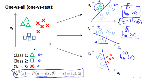
上图可知我们先取一个 class 进行计算，将其他的归类为另一个 class，这样就可以使用前面提到的 binary regression model 进行计算，即

\begin{aligned} y \in {0, 1 . . . n} \\ h_{θ}^{(0)} (x) = P (y = 0 | x; θ) \\ h_{θ}^{(1)} (x) = P (y = 1 | x; θ) \\ \dots \\ h_{θ}^{(n)} (x) = P (y = n | x; θ) \\ p r e d i c t i o n = max_{i} (h_{θ}^{(i)} (x)) \end{aligned}

One-vs-all(one-vs-rest):

Train a logistic regression classifier $h_{θ}^{(i)} (x)$ for each class $i$ to predict the probability that $y = i$ .

On a new input $x$ , to make a prediction, pick the class $i$ that maximizes

总结一下就是对每种分类先计算他的 $h_{θ} (x)$ ，当有一个新的x需要分类时，选一个让 $h_{θ} (x)$ 值最大的分类器。

附录：Regularization

The problem of overfitting

以线性回归的预测房价为例，如下图所示：

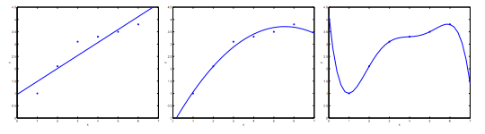
可以看到:

通过线性函数预测房价不够精确(underfit)，术语叫做”High Bias”，其原因主要是样本的 feature 太少了。
通过二次函数拟合出来的曲线刚好可以贯穿大部分数据样本，术语叫做”Just Right”
通过四阶多项式拟合出来的曲线虽然能贯穿所有数据样本，但是曲线本身不够规则，当有新样本出现时不能很好的预测。这种情况我们叫做Over Fitting（过度拟合），术语叫做”High variance”。If we have too many features, the learned hypothesis may fit the training set very well（J(θ)=0）, but fail to generalize to new examples(predict prices on new examples) Over Fitting 的问题在样本少，feature 多的时候很明显
Addressing overfitting: - Reduce number of features - Manually select which features to keep. - Model selection algorithm - Regularization - Keep all features, but reduce magnitude/values of parameters $θ_{j}$ - Works well when we have a lot of features, each of which contributes a bit to predicting $y$

Regularization Cost Function

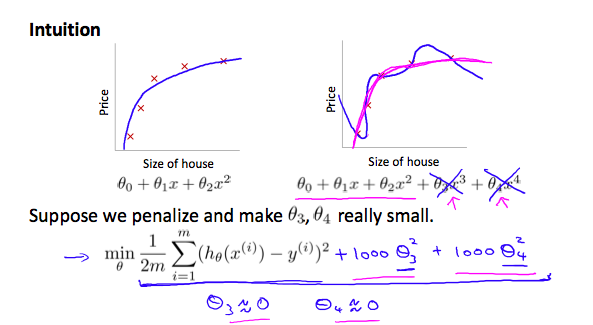
如果要减少 overfitting 的情况，我们可以降低一些参数的权重，假设我们想要让下面的函数变成二次方程：

θ_{0} + θ_{1} x + θ_{2} x^{2} + θ_{3} x^{3} + θ_{4} x^{4}

我们想要在不去掉 θ3 和 θ4 的前提下，降低 $θ_{3} x^{3}$ 和 $θ_{4} x^{4}$ 的影响，我们可以修改 cost function 为：

m i n_{θ} \frac{1}{2 m} \sum_{i = 1}^{m} (h_{θ} (x^{(i)}) - y^{(i)})^{2} + 1000 \cdot θ_{3}^{2} + 1000 \cdot θ_{4}^{2}

我们在原来的 cost function 后面增加了两项，为了让 cost function 接近 0，我们需要让 $θ_{3}$ , $θ_{4}$ 近似为 0，这样即会极大的减少 $θ_{3} x^{3}$ 和 $θ_{4} x^{4}$ 的值，减少后的曲线如下图粉色曲线，更接近二次函数：

Small values for parameters $θ_{0}, θ_{1},..., θ_{n}$

“Simpler” hypothesis，选取更小的θ值能得到更简单的预测函数，例如上面的例子，如果将 $θ_{3}, θ_{4}$ 近似为 0 的话，那么上述函数将变为二次方程，更贴近合理的假设函数
Housing example: - Feature: $x_{0}, x_{1},..., θ_{100}$ - Parameters: $θ_{0}, θ_{1},..., θ_{100}$

100 个 feature，如何有效的选取这些θ呢，改变 cost function：

J (θ) = \frac{1}{2 m} [\sum_{i = 1}^{m} (h_{θ} (x^{(i)}) - y^{(i)})^{2} + λ \sum_{j = 1}^{n} θ_{j}^{2}]

参数 λ 叫做regularization parameter，它的作用是既要保证曲线的拟合程度够高同时又要确保 θ 的值尽量小。如果 λ 的值选取过大，例如 $λ = 10^{10}$ ，会导致计算出的所有的 θ 值都接近 0，从而使 $h_{θ} (x) = θ_{0}$ 即产生”Under fitting”

Regularized linear regression

有了上面的式子，我们可以将它应用到线性回归：

修改梯度下降公式为：

\begin{aligned} Repeat { \\ θ_{0} := θ_{0} - α \frac{1}{m} \sum_{i = 1}^{m} (h_{θ} (x^{(i)}) - y^{(i)}) x_{0}^{(i)} \\ θ_{j} := θ_{j} - α [(\frac{1}{m} \sum_{i = 1}^{m} (h_{θ} (x^{(i)}) - y^{(i)}) x_{j}^{(i)}) + \frac{λ}{m} θ_{j}] & j \in {1, 2... n} \\ } \end{aligned}

将 $\frac{λ}{m} θ_{j}$ 提出来，得到:

θ_{j} := θ_{j} (1 - α \frac{λ}{m}) - α \frac{1}{m} \sum_{i = 1}^{m} (h_{θ} (x^{(i)}) - y^{(i)}) x_{j}^{(i)}

上述式子中 $1 - α \frac{λ}{m}$ 必须小于 1，这样就减小了 $θ_{j}$ 的值，后面的式子和之前梯度下降的式子相同

应用到 Normal Equation

和之前的公式相比，增加了一项：

\begin{aligned} θ = {(X^{T} X + λ \cdot L)}^{- 1} X^{T} y \\ where L = [\begin{matrix} 0 \\ 1 \\ 1 \\ ⋱ \\ 1 \end{matrix}] \end{aligned}

L 是一个（n+1)x(n+1)的对单位阵，第一项是 0。在引入 λ.L 之后 $X^{T} X + λ L$ 保证可逆

Regularized logistic regression

逻辑回归也有 overfitting 的问题，如图所示

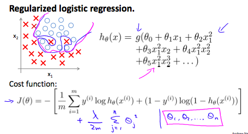
处理方式和线性回归相同，之前知道逻辑回归的 cost function 如下：

J (θ) = - \frac{1}{m} \sum_{i = 1}^{m} [y^{(i)} \log (h_{θ} (x^{(i)})) + (1 - y^{(i)}) \log (1 - h_{θ} (x^{(i)}))]

我们可以在最后加一项来 regularize 这个函数：

J (θ) = - \frac{1}{m} \sum_{i = 1}^{m} [y^{(i)} \log (h_{θ} (x^{(i)})) + (1 - y^{(i)}) \log (1 - h_{θ} (x^{(i)}))] + \frac{λ}{2 m} \sum_{j = 1}^{n} θ_{j}^{2}

第二项： $\sum_{j = 1}^{n} θ_{j}^{2}$ 是排除了 $θ_{0}$ 的，因此，计算梯度下降要对 $θ_{0}$ 单独计算:

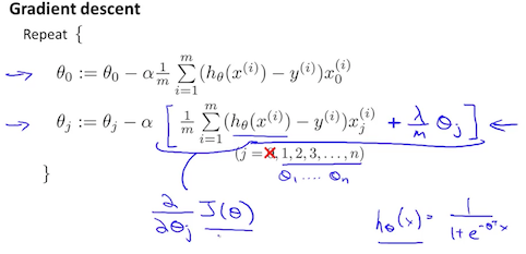
Octave Demo

function [J, grad] = lrCostFunction(theta, X, y, lambda{

%LRCOSTFUNCTION Compute cost and gradient for logistic regression with
%regularization
%   J = LRCOSTFUNCTION(theta, X, y, lambda) computes the cost of using
%   theta as the parameter for regularized logistic regression and the
%   gradient of the cost w.r.t. to the parameters.

% Initialize some useful values
m = length(y); % number of training examples

% You need to return the following variables correctly
J = 0;
grad = zeros(size(theta));



h = sigmoid(X*theta); %  X:118x28, theta:28x1 h:118x1

%向量化实现
J = 1/m * (-y'*log(h)-(1-y)'*log(1-h)) + 0.5*lambda/m * sum(theta([2:end]).^2);
%代数形式实现
%J = 1/m * sum((-y).*log(h) - (1-y).*log(1-h)) + 0.5*lambda/m * sum(theta([2:end]).^2);

grad = 1/m * X'*(h-y);

r = lambda/m .* theta;
r(1) = 0; %skip theta(0)
grad = grad + r;


% =============================================================

grad = grad(:);

}

function g = sigmoid(z)
	g = 1.0 ./ (1.0 + exp(-z));
end