
Shallow Neural Networks
文中部分图片截取自课程视频Nerual Networks and Deep Learning
Notations
- $x^{(i)}$:表示第$i$组训练样本
- $x^{(i)}_j$:表示第$i$组训练样本的第$j$个 feature
- $a^{[l]}$:表示第$l$层神经网络
- $a^{[l]}_i$: 表示第$l$层神经网络的第$i$个节点
- $a^{[l] (m)}_i$:表示第$m$个训练样本的第$l$层神经网络的第$i$个节点
单神经网络
遵循上述的 Notation,一个只有一组训练样本的$(x_1, x_2, x_3)$的两层神经网络可用下图描述
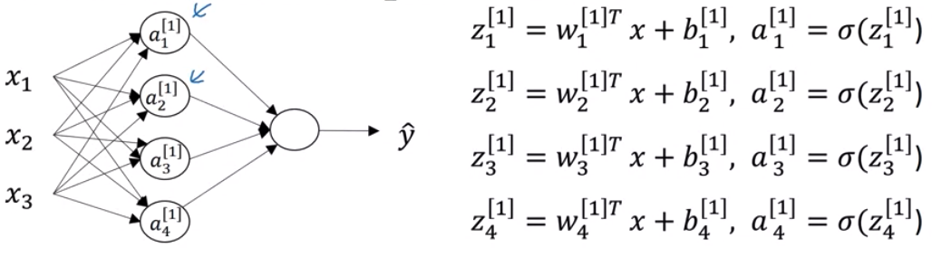
将上述式子用向量表示,则对于给定的输入$x$,有
\[\begin{align*} & z^{[1]} = W^{[1]}x + b^{[1]} \\ & a^{[1]} = \sigma(z^{[1]}) \\ & z^{[2]} = W^{[2]}a^{[1]} + b^{[2]} \\ & a^{[2]} = \sigma(z^{[2]}) \end{align*}\]其中,
- $z^{[1]}$是
4x1,$W^{[1]}$是4x3,$x$是3x1,$b^{[1]}$是4x1,$a^{[1]}$是4x1 - $z^{[2]}$是
1x1,$W^{[2]}$是1x4,$a^{[2]}$是1x1,$b^{[2]}$是1x1
Forward Propagation
上述神经网络只有一个组训练集,如果将训练集扩展到多组($x^{(1)}$,$x^{(2)}$,…,$x^{(m)}$),则我们需要一个for循环来实现每组样本的神经网络计算,然后对它们进行求和
结合前面文章可知,我们可以用向量化计算来取代for循环,另
则上述两层神经网络的向量化表示为
\[\begin{align*} & Z^{[1]} = W^{[1]}X + b^{[1]} \\ & A^{[1]} = \sigma(Z^{[1]}) \\ & Z^{[2]} = W^{[2]}A^{[1]} + b^{[2]} \\ & A^{[2]} = \sigma(Z^{[2]}) \end{align*}\]其中,$X$是3xm, $W^{[1]}$依旧是4x3, $A^{[i]}$是4xm,$b^{[1]}$也是4xm, $W^{[2]}$是3x1,$A^{[2]}$是1xm, $b^{[2]}$是1xm的。由此可以看出,训练样本增加并不影响$W^{[1]}$的维度
Activation Functions
如果神经网路的某个 Layer 要求输出结果在[0,1]之间,那么选取$\sigma(x) = \frac{1}{1+e^{-x}}$作为 Activation 函数,此外,则可以使用Rectified Linear Unit函数:
实际上可选择的 Activation 函数有很多种,但它们需要具备下面的条件
- 必须是非线性的
- 需要可微分,可计算梯度
- 需要有一个变化 sensitive 的区域和一个非 sensitive 的区域
总的来说 Activation 函数的作用在于通过非线性变换,让神经网络易于训练,可以更好的适应梯度下降
Back Propagation
上述神经网络的 Cost 函数和前文一样
\[J(W^{[1]}, b^{[1]}, W^{[2]}, b^{[2]}) = \frac {1}{m} \sum_{i=1}^{m}L(\hat{y}, y) =-\frac{1}{m} \sum_{i = 1}^{m} (y^{(i)}\log(A^{[2] (i)}) + (1-y^{(i)})\log(1- A^{[2] (i)}))\]其中$Y$为1xm的行向量 $Y = [y^{[1]},y^{[2]},…,y^{[m]}]$。按照上一节介绍的链式求导法则,对上述 Cost 函数求导,可以得出下面结论(推导过程省略)
- $dZ^{[2]} = A^{[2]} - Y$
- $dW^{[2]} = \frac{1}{m}dZ^{[2]}A^{[1]^{T}}$
- $db^{[2]} = \frac{1}{m}np.sum(dz^{[2]}, axis=1, keepdims=True)$
- $dz^{[1]} = W^{[2]^{T}}dZ^{[2]} * g^{[1]’}(Z^{[1]}) \quad (element-wise \ product)$
- $dW^{[1]} = \frac{1}{m}dZ^{[1]}X^{T}$
- $db^{[1]} = \frac{1}{m}np.sum(dz^{[1]}, axis=1, keepdims=True)$
其中$g^{[1]’}(Z^{[1]})$取决于 Activation 函数的选取,如果使用$tanh$,则$g^{[1]’}(Z^{[1]}) = 1-A^{[1]^2}$
Gradient Descent
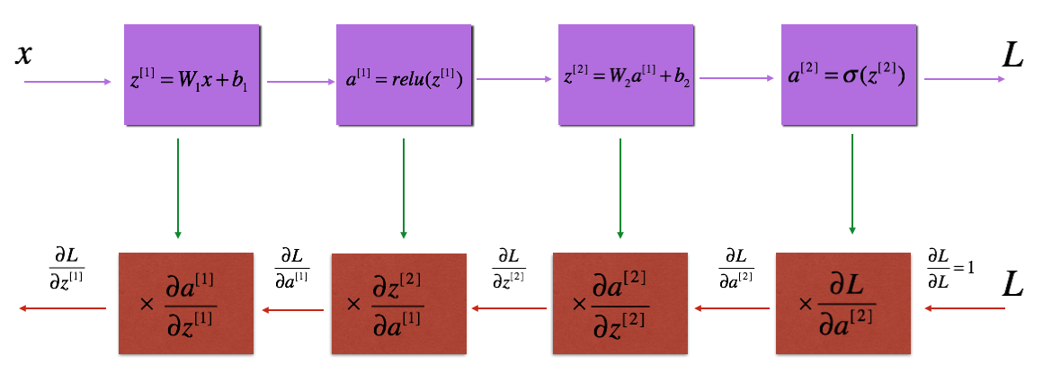
有了$dW^{[2]}$,$dW^{[1]}$,$db^{[2]}$,$db^{[2]}$的计算公式,我们变可以使用梯度下降来求解 $W^{[1]}, b^{[1]}, W^{[2]}, b^{[2]}$了,其反向求导的过程如下图所示
在每次 BP 完成后,我们需要对$dw$和$db$进行梯度下降
\[\begin{align*} & W^{[l]} = W^{[l]} - \alpha \text{ } dW^{[l]} \\ & b^{[l]} = b^{[l]} - \alpha \text{ } db^{[l]} \end{align*}\]其中对$\alpha$的取值需要注意,不同 learning rate 的选取对梯度下降收敛的速度有着重要的影响,如下图
Resources
附录: Numpy 实现
接下来我们用 numpy 来实现一个两层的神经网络,第一层的 activation 函数为 Relu,第二层为 Sigmoid。
- Initialization
第一步我们来初始化$W$和$b$,我们使用np.random.randn(shape)*0.01来初始化$W$,使用np.zeros来初始化$b$
def initialize_parameters(n_x, n_h, n_y):
    """
    Argument:
    n_x -- size of the input layer
    n_h -- size of the hidden layer
    n_y -- size of the output layer

    Returns:
    parameters -- python dictionary containing your parameters:
                    W1 -- weight matrix of shape (n_h, n_x)
                    b1 -- bias vector of shape (n_h, 1)
                    W2 -- weight matrix of shape (n_y, n_h)
                    b2 -- bias vector of shape (n_y, 1)
    """

    np.random.seed(1)

    W1 = np.random.randn(n_h,n_x) * 0.01
    b1 = np.zeros((n_h,1))
    W2 = np.random.randn(n_y,n_h) * 0.01
    b2 = np.zeros((n_y,1))

    parameters = {"W1": W1,
                  "b1": b1,
                  "W2": W2,
                  "b2": b2}

    return parameters
- Forward Propagation
参数初始化完成后,我们可以来实现 FP 了,其公式为
\[Z^{[l]} = W^{[l]}A^{[l-1]} +b^{[l]}\tag{4}\]为了后面便于计算 back prop,我们会将 FP 的计算结果缓存起来
def linear_forward(A, W, b):
    """
    Implement the linear part of a layer's forward propagation.

    Arguments:
    A -- activations from previous layer (or input data): (size of previous layer, number of examples)
    W -- weights matrix: numpy array of shape (size of current layer, size of previous layer)
    b -- bias vector, numpy array of shape (size of the current layer, 1)

    Returns:
    Z -- the input of the activation function, also called pre-activation parameter
    cache -- a python tuple containing "A", "W" and "b" ; stored for computing the backward pass efficiently
    """

    Z = np.dot(W,A) + b
    cache = (A, W, b)

    return Z, cache

def linear_activation_forward(A_prev, W, b, activation):
    """
    Implement the forward propagation for the LINEAR->ACTIVATION layer

    Arguments:
    A_prev -- activations from previous layer (or input data): (size of previous layer, number of examples)
    W -- weights matrix: numpy array of shape (size of current layer, size of previous layer)
    b -- bias vector, numpy array of shape (size of the current layer, 1)
    activation -- the activation to be used in this layer, stored as a text string: "sigmoid" or "relu"

    Returns:
    A -- the output of the activation function, also called the post-activation value
    cache -- a python tuple containing "linear_cache" and "activation_cache";
             stored for computing the backward pass efficiently
    """

    if activation == "sigmoid":
        # Inputs: "A_prev, W, b". Outputs: "A, activation_cache".
        Z, linear_cache = linear_forward(A_prev, W, b)
        A, activation_cache = sigmoid(Z)

    elif activation == "relu":
        # Inputs: "A_prev, W, b". Outputs: "A, activation_cache".
        Z, linear_cache = linear_forward(A_prev, W, b)
        A, activation_cache = relu(Z)

    cache = (linear_cache, activation_cache)
    return A, cache
- Cost Function
回顾计算 Cost 函数的公式如下
\[-\frac{1}{m} \sum\limits_{i = 1}^{m} (y^{(i)}\log\left(a^{[L] (i)}\right) + (1-y^{(i)})\log\left(1- a^{[L](i)}\right))\]def compute_cost(AL, Y):
"""
Implement the cost function defined by equation (7).
Arguments:
AL -- probability vector corresponding to your label predictions, shape (1, number of examples)
Y -- true "label" vector (for example: containing 0 if non-cat, 1 if cat), shape (1, number of examples)
Returns:
cost -- cross-entropy cost
"""
m = Y.shape[1]
# Compute loss from aL and y.
cost = -1/m *(np.dot(Y, np.log(AL.T)) + np.dot(1-Y, np.log(1-AL).T))
# To make sure your cost's shape is what we expect (e.g. this turns [[17]] into 17).
cost = np.squeeze(cost)
assert(cost.shape == ())
return cost
- Backward propagation
对于两层的神经网络,其反向求导的过程如下图所示
对于第$l$层网络,FP 得到的结果为$Z^{[l]} = W^{[l]} A^{[l-1]} + b^{[l]}$, 假设我们已经知道 $dZ^{[l]} = \frac{\partial \mathcal{L} }{\partial Z^{[l]}}$ 的值,我们的目的是求出 $(dW^{[l]}, db^{[l]}, dA^{[l-1]})$,如下图所示
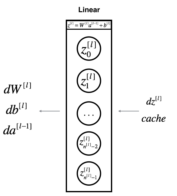
其中$dZ^{[l]}$的计算公式前面已经给出
\[dZ^{[l]} = dA^{[l]} * g'(Z^{[l]}) \tag{11}\]numpy 内置了求解dz的函数,我们可以直接使用
## sigmoid
dZ = sigmoid_backward(dA, activation_cache)
## relu
dZ = relu_backward(dA, activation_cache)
$dW^{[l]}, db^{[l]}, dA^{[l-1]}$的计算可参考前面小结给出的公式
def linear_backward(dZ, cache):
    """
    Implement the linear portion of backward propagation for a single layer (layer l)

    Arguments:
    dZ -- Gradient of the cost with respect to the linear output (of current layer l)
    cache -- tuple of values (A_prev, W, b) coming from the forward propagation in the current layer

    Returns:
    dA_prev -- Gradient of the cost with respect to the activation (of the previous layer l-1), same shape as A_prev
    dW -- Gradient of the cost with respect to W (current layer l), same shape as W
    db -- Gradient of the cost with respect to b (current layer l), same shape as b
    """
    A_prev, W, b = cache
    m = A_prev.shape[1]

    dW = 1/m * np.dot(dZ, A_prev.T)
    db = 1/m * np.sum(dZ, axis = 1, keepdims = True)
    dA_prev = np.dot(W.T, dZ)

    assert (dA_prev.shape == A_prev.shape)
    assert (dW.shape == W.shape)
    assert (db.shape == b.shape)

    return dA_prev, dW, db

def linear_activation_backward(dA, cache, activation):
    """
    Implement the backward propagation for the LINEAR->ACTIVATION layer.

    Arguments:
    dA -- post-activation gradient for current layer l
    cache -- tuple of values (linear_cache, activation_cache) we store for computing backward propagation efficiently
    activation -- the activation to be used in this layer, stored as a text string: "sigmoid" or "relu"

    Returns:
    dA_prev -- Gradient of the cost with respect to the activation (of the previous layer l-1), same shape as A_prev
    dW -- Gradient of the cost with respect to W (current layer l), same shape as W
    db -- Gradient of the cost with respect to b (current layer l), same shape as b
    """
    linear_cache, activation_cache = cache

    if activation == "relu":
        dZ = relu_backward(dA,activation_cache)
        dA_prev, dW, db = linear_backward(dZ,linear_cache)

    elif activation == "sigmoid":
        dZ = sigmoid_backward(dA,activation_cache)
        dA_prev, dW, db = linear_backward(dZ,linear_cache)

    return dA_prev, dW, db
- Update Parameters
在每次 BP 完成后,我们需要对$dw$h 和$db$进行梯度下降
\[\begin{align*} & W^{[l]} = W^{[l]} - \alpha \text{ } dW^{[l]} \\ & b^{[l]} = b^{[l]} - \alpha \text{ } db^{[l]} \end{align*}\]
def update_parameters(parameters, grads, learning_rate):
    """
    Update parameters using gradient descent

    Arguments:
    parameters -- python dictionary containing your parameters
    grads -- python dictionary containing your gradients, output of L_model_backward

    Returns:
    parameters -- python dictionary containing your updated parameters
                  parameters["W" + str(l)] = ...
                  parameters["b" + str(l)] = ...
    """

    L = len(parameters) // 2 # number of layers in the neural network
    # Update rule for each parameter. Use a for loop.
    for l in range(L):
        parameters["W" + str(l+1)] = parameters["W" + str(l+1)] - learning_rate * grads["dW"+str(l+1)]
        parameters["b" + str(l+1)] = parameters["b" + str(l+1)] - learning_rate * grads["db"+str(l+1)]
    return parameters