Deep Neural Networks

Posted on 2018-01-28 | In AI , Machine Learning , Deep Learning

文中部分图片截取自课程视频Nerual Networks and Deep Learning

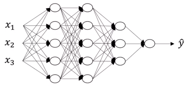
Now we have a better understanding of how the two-layer neural networks works, we can apply and extend the idea to any multi-layer neural network.

Notations

$n^{[l]}$: #units in layer $l$
$a^{[l]}$: #activations units in layer $l$
- $a^{[l]}=g^{[l]}(z^{[l]})$
- $a^{[0]} = X$
$W^{[l]}$: weights for $z^{[l]}$
$b^{[l]}$: bias vector

Forward Propagation for Layer $l$

Input $a^{[l-1]}$
Output $a^{[l]}$, cache (z^{[l]})

\[\begin{align*} & Z^{[l]} = W^{[l]}A^{[l-1]} + $b^{[l]} \\ & A^{[l]} = g^{[l]}(Z^{[l]}) \\ \end{align*}\]

其中，$W^{[l]}$矩阵的维度为$(n^{[l]}, n^{[l-1]})$, $b^{[l]}$的维度为$(n^{[l]},1)$，$Z^{[l]}$和$A^{[l]}$均为$(n^{[l]},m)$ （m为训练样本数量）

Although we can use vectorization to compute $A^{[l]}$ more easily, we still need to use a explicit for-loop to loop thourgh all the hidden layers, as the deep neural networks always have more than one layers.

Backward Propagation for layer $l$

Input $da^{[l]}$
Output $da^{[l-1]}$, $dW^{[l]}$, $db^{[l]}$

\[\begin{align*} & dz^{[l]} = da^{[l]} * g^{[l]'}(z^{[l]}) \quad (element-wise \ product) \\ & dw^{[l]} = dz^{[l]}a^{[l-1]} \\ & db^{[l]} = dz^{[1]} \\ & da^{[l-1]} = w^{[l]^T}dz^{[l]} \\ \end{align*}\]

Vetorized version

\[\begin{align*} & dZ^{[l]} = dA^{[l]} * g'(Z^{[l]}) \quad (element-wise \ product) \\ & dW^{[l]} = \frac{1}{m}dZ^{[l]}A^{[l-1]^T} \\ & db^{[l]} = \frac{1}{m}np.sum(dZ^{[l]}, axis=1, keepdims=True) \\ & dA^{[l-1]} = W^{[l]^T}dZ^{[l]} \\ \end{align*}\]

Hyperparameters

learning rate $\alpha$
#iterations
#hidden layer
#hidden units
choice of activation function
…

Build a Multilayer Neural Networks in Numpy

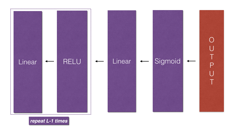
和前一篇文章类似，接下来我们将用numpy来实现一个L层的神经网络。我们另前$L-1$层的Activation函数为Relu，最后一层的Activation函数为Sigmoid。

Initialization

def initialize_parameters_deep(layer_dims):
    """
    Arguments:
    layer_dims -- python array (list) containing the dimensions of each layer in our network
    
    Returns:
    parameters -- python dictionary containing your parameters "W1", "b1", ..., "WL", "bL":
                    Wl -- weight matrix of shape (layer_dims[l], layer_dims[l-1])
                    bl -- bias vector of shape (layer_dims[l], 1)
    """
    
    np.random.seed(3)
    parameters = {}
    L = len(layer_dims)            # number of layers in the network

    for l in range(1, L):
        parameters['W' + str(l)] = np.random.rand(layer_dims[l], layer_dims[l-1]) * 0.01
        parameters['b' + str(l)] = np.zeros((layer_dims[l], 1))


    return parameters

参数初始化完成后，我们可以来实现FP了，借助前一篇两层神经网络的linear_forward和linear_activation_forward函数，我们可以方便的实现第$L$层的forward

def L_model_forward(X, parameters):
    """
    Implement forward propagation for the [LINEAR->RELU]*(L-1)->LINEAR->SIGMOID computation
    
    Arguments:
    X -- data, numpy array of shape (input size, number of examples)
    parameters -- output of initialize_parameters_deep()
    
    Returns:
    AL -- last post-activation value
    caches -- list of caches containing:
                every cache of linear_activation_forward() (there are L-1 of them, indexed from 0 to L-1)
    """

    caches = []
    A = X
    L = len(parameters) // 2                  # number of layers in the neural network    
    # Implement [LINEAR -> RELU]*(L-1). Add "cache" to the "caches" list.
    for l in range(1, L):
        A_prev = A 
        A, cache = linear_activation_forward(A_prev, parameters["W"+str(l)], parameters["b"+str(l)], "relu")
        caches.append(cache)
    
    # Implement LINEAR -> SIGMOID. Add "cache" to the "caches" list.
    AL, cache = linear_activation_forward(A, parameters["W"+str(L)], parameters["b"+str(L)], "sigmoid")
    caches.append(cache)

    assert(AL.shape == (1,X.shape[1]))
            
    return AL, caches

Cost Function

回顾计算Cost函数的公式如下

\[-\frac{1}{m} \sum\limits_{i = 1}^{m} (y^{(i)}\log\left(a^{[L] (i)}\right) + (1-y^{(i)})\log\left(1- a^{[L](i)}\right)) \tag{7}\]

def compute_cost(AL, Y):
    """
    Implement the cost function defined by equation (7).

    Arguments:
    AL -- probability vector corresponding to your label predictions, shape (1, number of examples)
    Y -- true "label" vector (for example: containing 0 if non-cat, 1 if cat), shape (1, number of examples)

    Returns:
    cost -- cross-entropy cost
    """
    m = Y.shape[1]
    # Compute loss from aL and y.
    cost = -1/m *(np.dot(Y, np.log(AL.T)) + np.dot(1-Y, np.log(1-AL).T))    
    # To make sure your cost's shape is what we expect (e.g. this turns [[17]] into 17).
    cost = np.squeeze(cost)      
    assert(cost.shape == ())
    return cost

Backward propagation

上面我们通过了L_model_forward对每层进行FB运算，并且缓存了(X,W,b, and z)。接下来我们便可以用这些缓存的结果进行反向求导。我们知道最后一层的输出结果为$A^{[L]} = \sigma(Z^{[L]})$，因此我们首先需要计算的是 $= \frac{\partial \mathcal{L}}{\partial A^{[L]}}$

# derivative of cost with respect to AL
dAL = - (np.divide(Y, AL) - np.divide(1 - Y, 1 - AL))

接下来我们便可以使用dAL对sigmoid函数求导得出$dW^{[l]}$,$db^{[l]}$,$dA^{[l-1]}$，接下来通过一个for循环，逐层求解$dw$,$db$和$dA$，如下图所示

在反向求导的过程中，我们需要将dA,dW和db缓存起来，便于后续梯度下降运算

def L_model_backward(AL, Y, caches):
    """
    Implement the backward propagation for the [LINEAR->RELU] * (L-1) -> LINEAR -> SIGMOID group
    
    Arguments:
    AL -- probability vector, output of the forward propagation (L_model_forward())
    Y -- true "label" vector (containing 0 if non-cat, 1 if cat)
    caches -- list of caches containing:
                every cache of linear_activation_forward() with "relu" (it's caches[l], for l in range(L-1) i.e l = 0...L-2)
                the cache of linear_activation_forward() with "sigmoid" (it's caches[L-1])
    
    Returns:
    grads -- A dictionary with the gradients
             grads["dA" + str(l)] = ... 
             grads["dW" + str(l)] = ...
             grads["db" + str(l)] = ... 
    """
    grads = {}
    L = len(caches) # the number of layers
    m = AL.shape[1]
    Y = Y.reshape(AL.shape) # after this line, Y is the same shape as AL
    # Initializing the backpropagation
    dAL = - (np.divide(Y, AL) - np.divide(1 - Y, 1 - AL))
    # Lth layer (SIGMOID -> LINEAR) gradients. Inputs: "dAL, current_cache". Outputs: "grads["dAL-1"], grads["dWL"], grads["dbL"]
    current_cache = caches[L-1]
    grads["dA" + str(L-1)], grads["dW" + str(L)], grads["db" + str(L)] = linear_activation_backward(dAL, current_cache, activation = "sigmoid")
    # Loop from l=L-2 to l=0
    for l in reversed(range(L-1)):
        # lth layer: (RELU -> LINEAR) gradients.
        # Inputs: "grads["dA" + str(l + 1)], current_cache". Outputs: "grads["dA" + str(l)] , grads["dW" + str(l + 1)] , grads["db" + str(l + 1)] 
        current_cache = caches[l]
        dA_prev_temp, dW_temp, db_temp = linear_activation_backward(grads["dA" + str(l+1)], current_cache, activation = "relu")
        grads["dA" + str(l)] = dA_prev_temp
        grads["dW" + str(l + 1)] = dW_temp
        grads["db" + str(l + 1)] = db_temp

    return grads

Update Parameters

在每次BP完成后，我们需要对$dw$h和$db$进行梯度下降

\[\begin{align*} & W^{[l]} = W^{[l]} - \alpha \text{ } dW^{[l]} \\ & b^{[l]} = b^{[l]} - \alpha \text{ } db^{[l]} \end{align*}\]

def update_parameters(parameters, grads, learning_rate):
    """
    Update parameters using gradient descent
    
    Arguments:
    parameters -- python dictionary containing your parameters 
    grads -- python dictionary containing your gradients, output of L_model_backward
    
    Returns:
    parameters -- python dictionary containing your updated parameters 
                  parameters["W" + str(l)] = ... 
                  parameters["b" + str(l)] = ...
    """
    
    L = len(parameters) // 2 # number of layers in the neural network
    # Update rule for each parameter. Use a for loop.
    for l in range(L):
        parameters["W" + str(l+1)] = parameters["W" + str(l+1)] - learning_rate * grads["dW"+str(l+1)]
        parameters["b" + str(l+1)] = parameters["b" + str(l+1)] - learning_rate * grads["db"+str(l+1)]
    return parameters