Hperparameters | Regularization

Posted on 2018-02-05 | In AI , Machine Learning , Deep Learning

Bias and Variance

如果我们在train data上面的error很低，但是在Dev set上的error很高，说明我们的模型出现over fitting，这种情况下我们说模型的Variance很高。如果二者错误率接近，且都很高，这是我们称为high bias，此时我们的模型的问题是under fitting。解决high bias可以引入更多的hidden layer来增加training的时间，或者使用一些的优化方法，后面会提到。如果要解决over fitting的问题，我们则需要更多的数据或者使用Regularization。

Regularization

我们还是用Logistic Regression来举例。在LR中，Cost Function定义为

$J(w,b) = \frac{1}{m}\sum_{i=1}^{m}L(\hat{y}^{(i)}, y^{(i)})$

为了解决Overfitting，我们可以在上面式子的末尾增加一个Regularization项

$J(w,b) = \frac{1}{m}\sum_{i=1}^{m}L(\hat{y}^{(i)}, y^{(i)}) + \frac{\lambda}{2m}||{w}||{^2}$

上述公式末尾的二范数也称作L2 Regularization，其中$\omega$的二范数定义为

$||{w}||{^2} = \sum_{j=1}^{n_x}\omega^{2}_{j} = \omega^T\omega$

除了使用L2范数外，也有些model使用L1范数，即$\frac{\lambda}{2m}||\omega||_1$。

如果使用L1范数，得到的$\omega$矩阵会较为稀疏（0很多），不常用。

对于一般的Neural Network，Cost Function定义为

$J(\omega^{[1]}, b^{[1]},...,\omega^{[l]}, b^{[l]}) = \frac{1}{m}\sum_{i=1}^{m}L(\hat{y^{(i)}}, y^{(i)}) + \frac{\lambda}{2m}||{\omega}||{^2}$

其中对于某$l$层的L2范数计算方法为

$||\omega^{[l]}||^{(2)} = \sum_{i=1}^{n^{l}}\sum_{j=1}^{n^{(l-1)}}(\omega_{i,j}^{[l]})^2$

其中$i$表示row，$n^{l}$表示当前层有多少neuron(输出)，$j$表示column，$n^{(l-1)}$为前一层的输入有多少个neuron。简单理解，上面的L2范数就是对权重矩阵中的每个元素平方后求和。

Python代码为

for l in range(1, L):
    L2_regularization_cost += (np.sum(np.square(Wl))
L2_regularization_cost = L2_regularization_cost * lambd/(2*m)

新增的Regularization项同样会对反响求导产生影响，我们同样需要增加该Regularization项对$\omega$的导数

$d\omega = (from \ backprop) + \frac{\lambda}{m}\omega$

Gradient Descent的公式不变

$\omega^{[l]} := \omega^{[l]} - \alpha d\omega^{[l]}$

将上面$d\omega$带入，可以得到

$\omega^{[l]} := \omega^{[l]} - \alpha[(from \ backprop) + \frac{\lambda}{m}\omega] = (1-\frac{\alpha\lambda}{m})\omega^{[l]} - \alpha(from \ backprop)$

可以看到，在引入正则项后，$\omega^{[l]}$实际上是减小了，因此，L2正则也称作weight decay。

引入正则项为什么能减少overfitting呢？我们可以从两方面来考虑。首先通过上面的式子可以看出，如果$\lambda$很大，则$\omega$会变小，极端情况下，会有一部分weights变成0，那么我们hidden units会减少，模型将变得简单。另一个思考的方式是看activation results，我们知道

$z^{[l]} = \omega^{[l]}\alpha^{[l-1]} + b^{[l]}$

当$\omega$变小后，$z$会变小，那么输出的结果将趋于于线性

Dropout

除了通过引入正则项来减少overfitting外，Dropout也是一种常用的手段。Dropout的思路很简单，每个hidden units将会以一定概率被去掉，去掉后的模型将变得更简单，从而减少overfitting。如下图所示

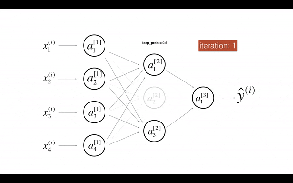
Dropout使Activation units不依赖前面layer某些具体的unit，从而使模型更加泛化。在实际应用中，Dropout比较流行的实现是inverted dropout，其思路为

产生一个bool矩阵, 以$l=3$为例
- d3 = (np.random.rand(a3.shape[0], a3.shape[1]) < keep_prob).astype(int)
- 其中keep_prob表示保留某个hidden unit的概率。则d3是一个0和1的bool矩阵
更新a3，根据keep_prob去掉某些units
- a3 = a3 * d3
Invert a3中的值。这么做相当于抵消掉去掉hidden units带来的影响
- a3 /= keep_prob

Numpy的伪代码如下

Z1 = np.dot(W1, X) + b1
A1 = relu(Z1)
D1 = np.random.rand(A1.shape[0], A1.shape[1])  # dropout matrix
D1 = (D1 < keep_prob).astype(int)  # dropout mask
A1 = A1*D1  # shut down some units in A1
A1 = A1/keep_prob  # scale the value of neurons that haven't been shut down

神经网络中每层的hidden units数量可能不同，keep_prob的值也可以根据其数量进行调整。Dropout表面上看起来很简单，但实际上它也属于Regularization的一种，具体证明就不展开了。需要注意的是，Dropout会影响back prop，由于hidden units会被随机cut off，Gradient Descent的收敛曲线也将会变得不规则。因此常用的手段一般是先另keep_prop=1，确保曲线收敛，然后再逐层调整keep_prop的值，重新训练。

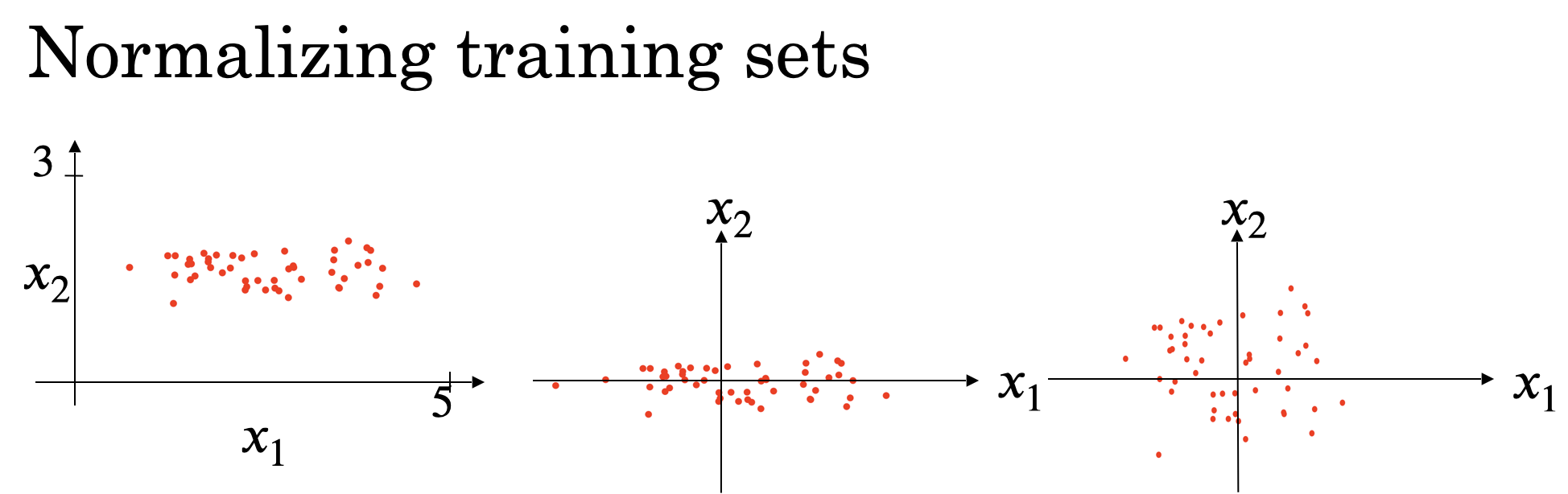
Normalizing Training Sets

对training数据 $X = [x_1, x_2]$，计算均值和方差

$\mu = \frac{1}{m}\sum_1^{m}x^{(i)} \\ x:=x-\mu \\ \sigma^2 = \frac{1}{m}\sum_1^{m}x^{(i)} ** 2 \\ x:=x / {\sigma^{2}} \\$

归一化前后的$x_1, x_2$分布如下图所示

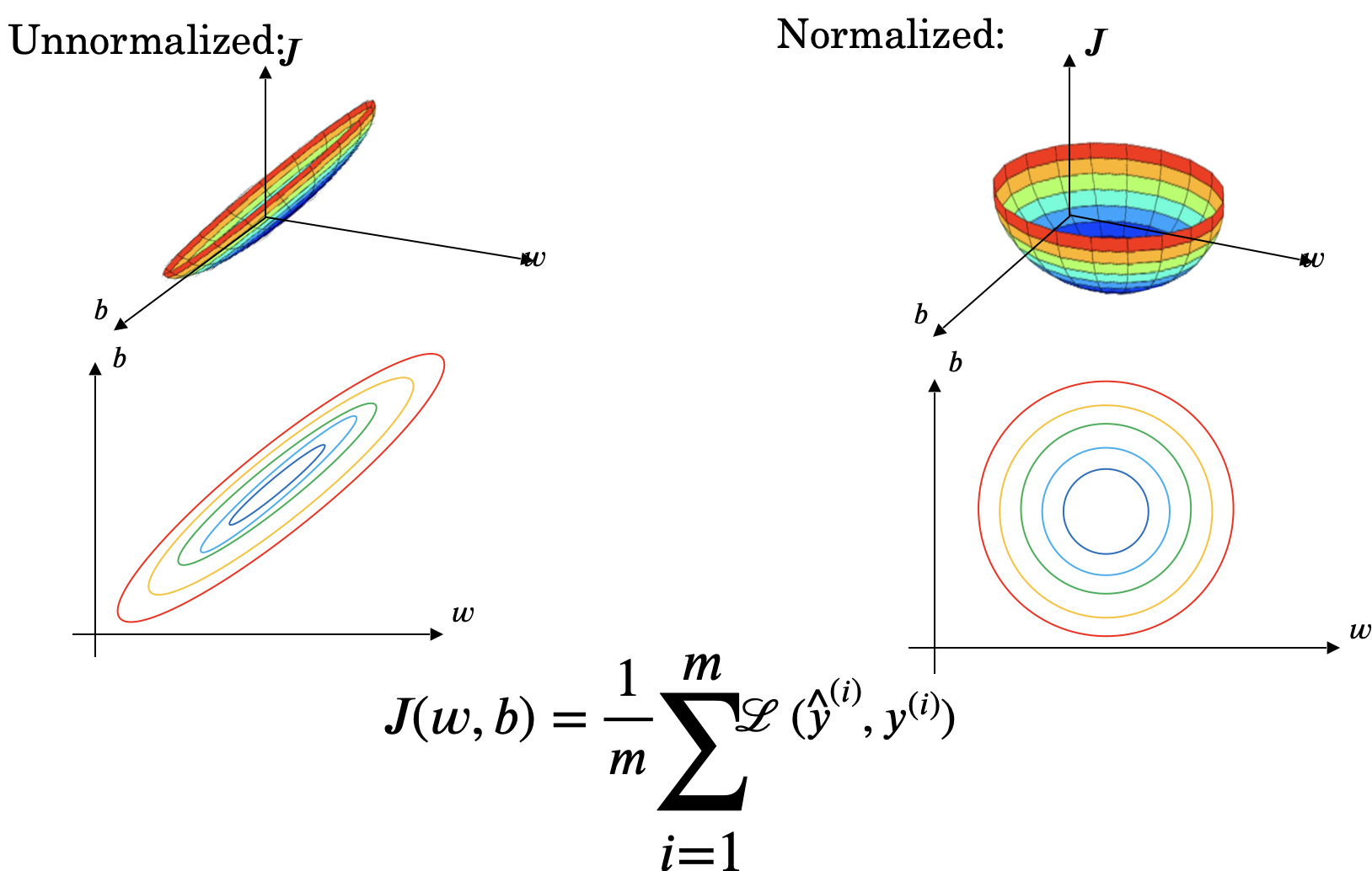
归一化training数据的目的是使training速度加快，因为Gradient Descent收敛加快，如下图所示

如果不同的feature数据之间scale比较大，比如0<x1<1000, 0<x2<1，此时将它们归一化将有更好的效果

Vanishing / Exploding gradients

梯度的消失和爆炸是指对于深层的神经网络，在training时导数值很大或者很小，从而导致training变得非常困难。假设我们有下面的network，它由$l$个full-connected layer组成

我们用$\omega^{[i]}$表示每层的weight值，简单起见，我们另activation函数为线性函数$g(z) = z$，另bias为0，则$\hat{y}$为

$\hat{y} = \omega^{[l]}\omega^{[l-1]}\omega^{[l-2]}...\omega^{[2]}\omega^{[1]}X$

我们假设每个$\omega^{[l]}$的值都为

$\begin{bmatrix} 1.5 & 0 \\ 0 & 1.5 \\ \end{bmatrix} or \begin{bmatrix} 0.5 & 0 \\ 0 & 0.5 \\ \end{bmatrix}$

则左边的矩阵，$a^{[l]}$将指数级增长。而对于右边矩阵，$\hat{y}$将指数级减小，这也会直接影响gradient descent的值（迭代很久，梯度只下降了一点点）。

Weight Initialization for deep networks

解决梯度爆炸或者消失的一种解决方法是对weight进行随机初始化。我们先看只有一个neuron的情况，如下图所示

我们暂时忽略bias，则$z=\omega_{1}x_{1}+\omega_{2}x_{2}+…+\omega_{n}x_{n}$

为了避免$z$过大或过小，我们一般用下面的方法对weight进行归一化

W[l] = np.random.rand(layers_dims[l]) * np.sqrt(2/(n**(l-1)))

上述式子会将weight的均值归一化到0左右，not too bigger than 1 and not too much less than 1。当activation函数为Relu的时候，这个方法比较有效。如果用tanh，则可以将np.sqrt(2/(n**(l-1))) 替换为np.sqrt(1/(n**(l-1)))。

Gradient checking

在bacKprop的过程中，如果我们不确定梯度计算的值是否准确，我们可以通过求导公式来验证

$\frac{\partial J}{\partial \theta} = \lim_{\varepsilon \to 0} \frac{J(\theta + \varepsilon) - J(\theta - \varepsilon)}{2 \varepsilon} \tag{1}$

具体做法是，将backprop过程中得到梯度值$\frac{\partial J}{\partial \theta}$和上述公式求出的梯度值进行比较。比较方法是根据下面公式计算误差值

$err = \frac{|| d\theta_{approx} - d\theta ||_2}{||d\theta_{approx}||_2 + ||d\theta||_2}$

一般误差的阈值为$\epsilon=10^{-7}$，则如果$err$能在$10^{-7}$左右说明，梯度计算正确，如果在$10^{-3}$则说明有较大的的问题。

Python的伪代码如下

def gradient_check(x, theta, epsilon = 1e-7):    
    thetaplus = theta + epsilon
    thetaminus = theta - epsilon
    J_plus = forward_propagation(x,thetaplus)
    J_minus = forward_propagation(x,thetaminus)
    gradapprox = (J_plus - J_minus) / (2*epsilon)
    
    # Check if gradapprox is close enough to the output of backward_propagation()
    grad = backward_propagation(x, theta)
    
    numerator = np.linalg.norm(grad - gradapprox)
    denominator = np.linalg.norm(grad) + np.linalg.norm(gradapprox)
    difference = numerator / denominator
    
    if difference < 1e-7:
        print ("The gradient is correct!")
    else:
        print ("The gradient is wrong!")
    return difference

假设我们有下面的network

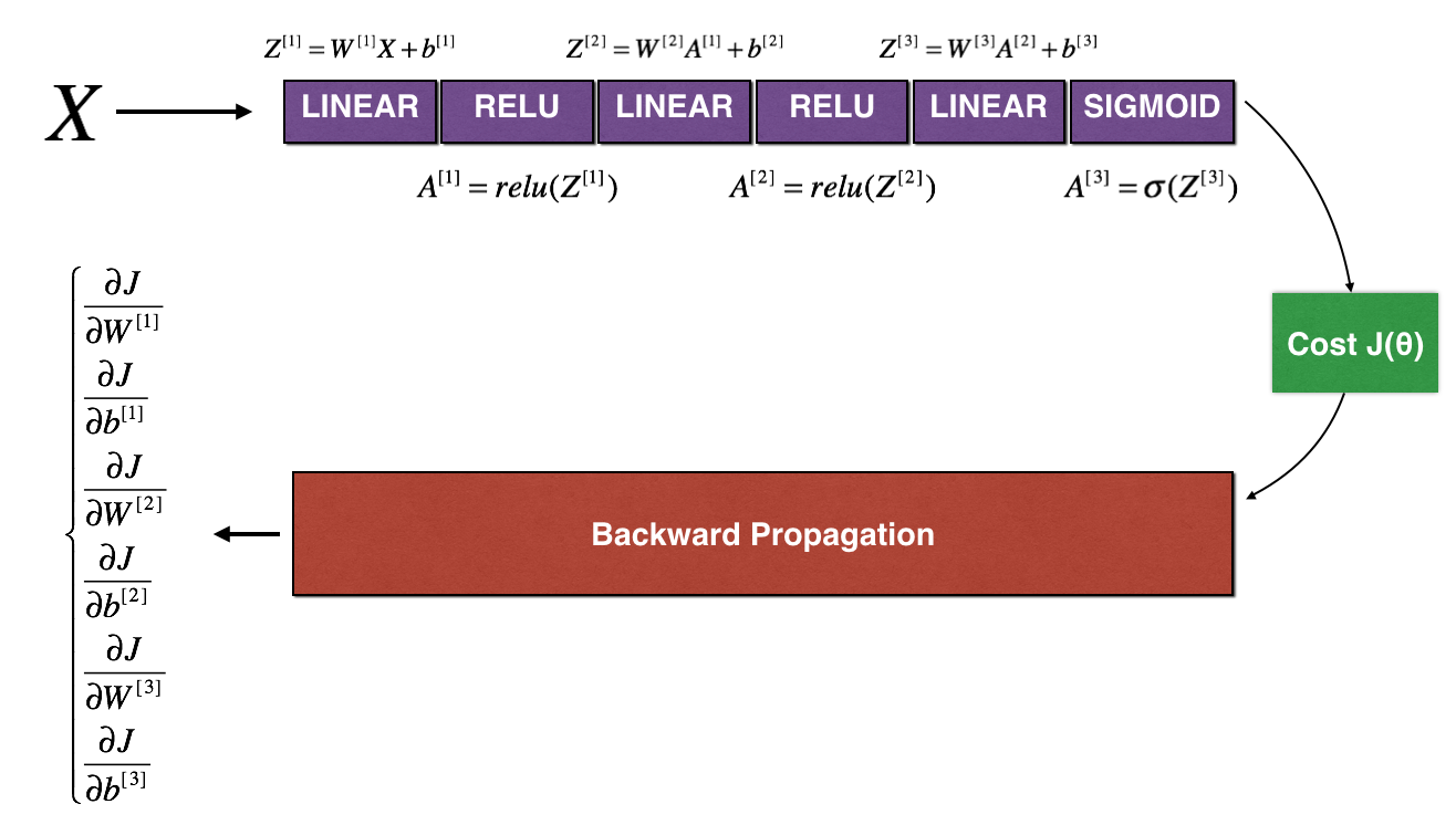
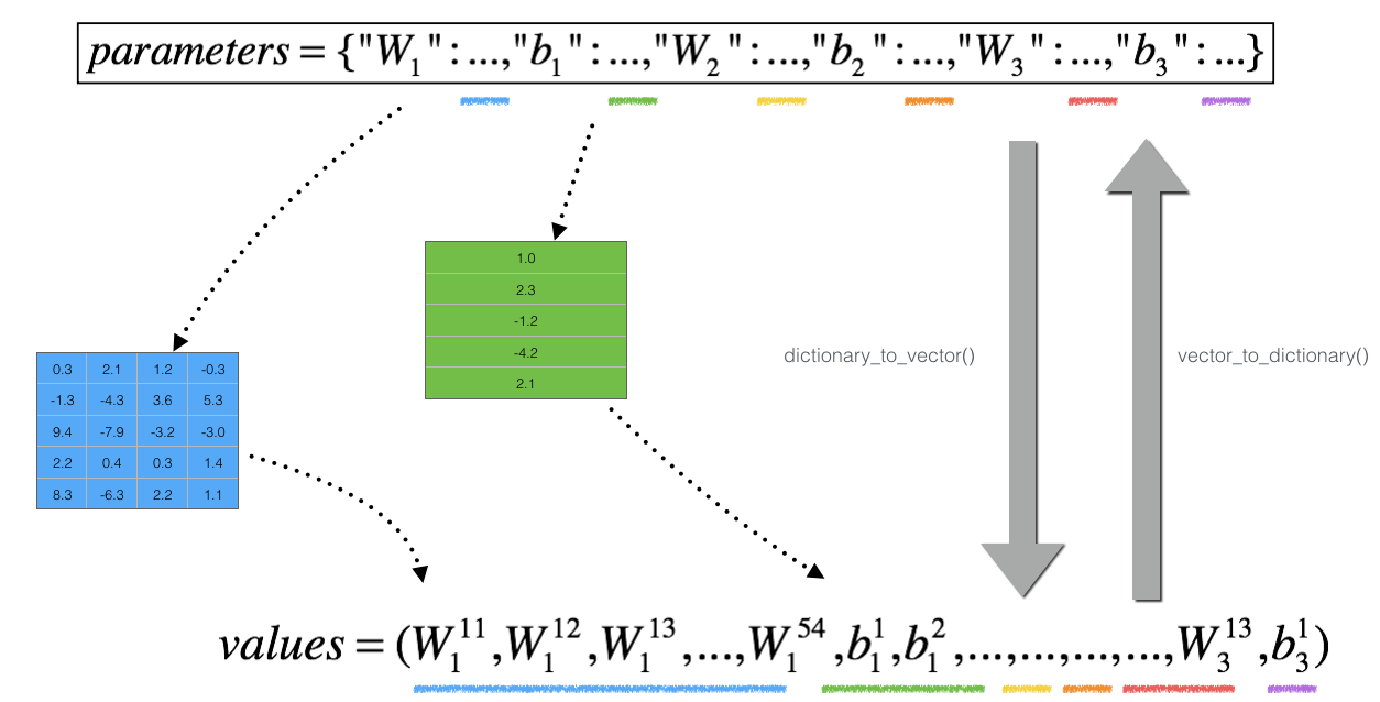
我们将 $W^{[1]},b^{[1]},W^{[2]},b^{[2]},W^{[3]},b^{[3]}$ 存到一个dictionary里并转为一个vector，称为 $\theta$, 如下图所示

则我们的cost函数变为

$J(W^{[1]},b^{[1]},...,W^{[L]},b^{[L]}) = J(\theta_1,\theta_2,...,\theta_L ) = J(\theta)$

相应的，我们也需要将$d\theta$存到一个vector里，即$[dW^{[1]},db^{[1]},dW^{[2]},db^{[2]},dW^{[3]},db^{[3]}]$

接下来我们执行下面步骤

计算J_plus[i]
- 计算$\theta^{+}$ = np.copy(parameters_values)
- $\theta^{+} = \theta^{+} + \epsilon$
- $J^{+}_i$ = forward_propagation_n(x, y, vector_to_dictionary(theta_plus))
重复上面步骤计算$\theta^{-}$和J_minus[i]
计算导数值 $gradapprox[i] = \frac{J^{+}_i - J^{-}_i}{2 \varepsilon}[i] = \frac{J^{+}_i - J^{-}_i}{2 \varepsilon}$

上述步骤完成后我们将得到一个gradapprox的vector，其中gradapprox[i]代表对parameter_values[i]的导数。接下来我们就可用上述误差函数来计算误差

Note
- Gradient Checking is slow! Approximating the gradient with $\frac{\partial J}{\partial \theta} \approx \frac{J(\theta + \varepsilon) - J(\theta - \varepsilon)}{2 \varepsilon}$ is computationally costly. For this reason, we don’t run gradient checking at every iteration during training. Just a few times to check if the gradient is correct.
- Gradient Checking, at least as we’ve presented it, doesn’t work with dropout. You would usually run the gradient check algorithm without dropout to make sure your backprop is correct, then add dropout.

Resource

Improving Deep Neural Networks: Hyperparameter tuning, Regularization and Optimization