
Optimization Algorithms
Mini-batch Gradient Descent
假设一组训练数据$X$有$m$个样本,$X = [x^{(1)},x^{(2)},x^{(3)},…,x^{(m)}]$,每个$x^{[i]}$有n个feature($X$的矩阵为$(n, m)$),相应的,$Y=[y^{(1)},y^{(2)},y^{(3)},…,y^{(m)}]$($Y$的矩阵大小为$(1, m)$)。对于m组数据,在training时,我们可以用vectorization的方式代替for循环,这样可以提高训练速度,我们称这种方式为Batch Gradient Descent。
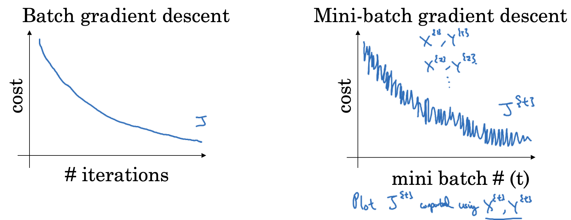
但是如果$m$非常大,比如5个million,那么将所有数据一起training,效率将非常低。实际上,在backprop的时候,我们不需要更新整个数据的weights和bias。我们可以将training set分成多个batch,比如将5个million切分成5000个小的batch,每个batch包含1000个训练数据。我们用 $X^{\text{{1}}}, Y^{\text{{1}}}$表示第1组mini batch, $X^{\text{{t}}}, Y^{\text{{t}}}$ 表示第$t$组训练数据。此时我们称为Mini-batch Gradient Descent
对training set的切分方式不同,会影响training的效率,表现为cost函数的收敛过程,如下图所示
如何选取mini batch的大小呢?
- 当batch size为
m的时候,称为Batch Gradient Descent,此时我们只有一个mini batch, 则有$(X^{\text{{1}}}, Y^{\text{{1}}}) = (X, Y)$ - 当batch size为
1的时候,称为Stochastic Gradient Descent,此时每一个training example都是一个单独的mini batch,则有$(X^{\text{{1}}}, Y^{\text{{1}}}) = (x^{(1)}, y^{(1)}), …, (X^{\text{{t}}}, Y^{\text{{t}}}) = (x^{(t)}, y^{(t)})$
三种方式的梯度下降过程如下图所示
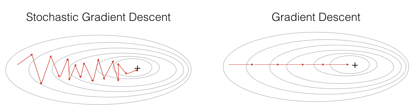
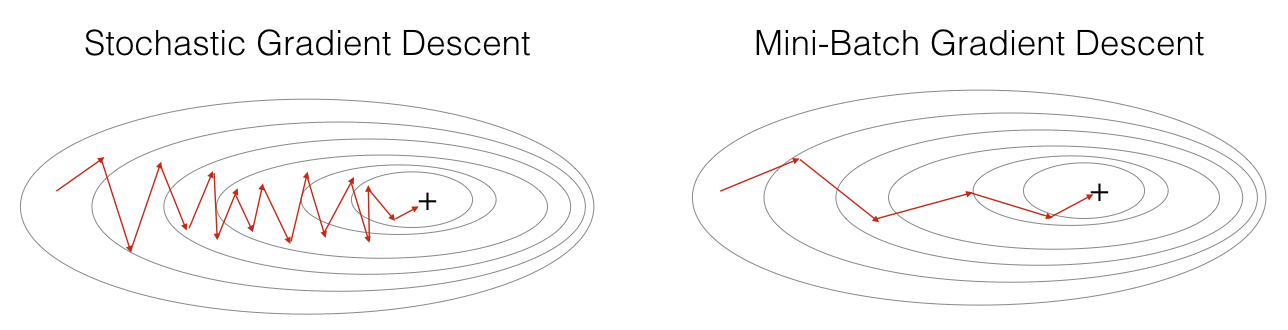
注意到,对于SGD,梯度下降的过程将极为noisy,这是由于在训练的过程中一个epoch只处理一个样本,失去了vectorization的并行处理能力。
在实际应用中,batch size往往在`(1, m)`中选取,可以参考如下策略:
- 如果训练样本很小(
m<2000),使用Batch Gradient Descent - 如果使用Mini Batch,
m可选取2的阶乘,比如64,128,256,512,1024 - 注意单个batch所产生的运算量(forward和backward)是否能被加载到当前的内存中
Exponentially Weighted Averages
除了Gradient Descent以外,还有一些其它的optimization算法可以加速model的训练过程,在介绍这些算法之前,我们需要先了解一下什么是Exponentially weighted averages。通俗来说Exponentially Weighted Averages是用来计算移动平均,计算方式如下
\[v_t = \beta v_{t-1} + (1-\beta) \theta_t\]其中$\beta$取值在0和1之间。我们用一个例子来说明其计算方式,下面是London一年的气温变化数据:
\[\begin{align*} \theta_1 &= 40^\circ \text{F} \\ \theta_2 &= 49^\circ \text{F} \\ \theta_3 &= 45^\circ \text{F} \\ &\vdots \\ \theta_{180} &= 60^\circ \text{F} \\ \theta_{181} &= 56^\circ \text{F} \end{align*}\]我们另$\beta$取值0.9,按照上面公式进行迭代计算,可得
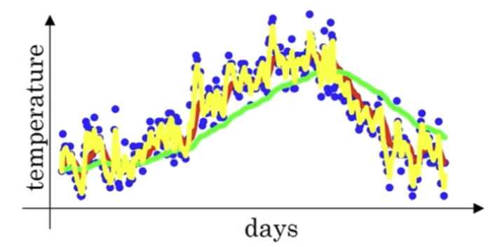
如果我们将计算结果绘制成曲线,我们可以得到下面红色的曲线:

由此可见,除了通过神经网络找到拟合曲线外,使用基于权重(weighted)的移动平均也能达到近似的目的,权重值即为$\beta$。实际上,当$\beta$的值越大,曲线越平滑,平均的样本数越多,反之则曲线越波动,平均样本越少。下图展示了当$\beta$为0.98(绿色),0.9和0.5(黄色)时的曲线变化。
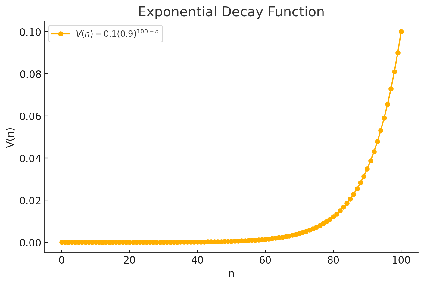
那为什么叫”Exponential” Weighted Average呢?这个指数从哪里来?让我们回到上面的例子中,如果我们另$t=100$,则有$v_{100} = 0.1\theta_{100} + 0.9v_{99}$, 而$v_{99} = 0.1\theta_{99} + 0.9v_{98}$,我们将$v_{98}$带入到$v_{99}$的式子中,将$v_{99}$带入到$v_{100}$的式子中,依次类推,能得到
\[v = 0.1 \theta_{100} + 0.1 \times 0.9 \theta_{99} + 0.1 (0.9)^2 \theta_{98} + \dots + 0.1 (0.9)^{100} \theta_0\]上面式子中,如果将自变量看成$\theta$,则$v$是一个指数函数,而且该函数所有项数之和约等于1:
上面式子中有一个问题是,起始阶段的值($v_0$, $v_1$…)会非常小,移动平均曲线并不能完整的反映训练样本的变化,因此实际应用中,如果我们关注这部分误差,我们可以用下面公式来计算移动平均,这个过程也叫做Bias Correction
\[\frac {v_t} {1-\beta^{t}}\]Gradient Descent with Momentum
使用基于动量(Momentum)的梯度下降会比传统的梯度下降速度快,它的工作原理是通过计算梯度的exponentially weighted averages值来更新神经网络的weights,从而实现加速。具体做法如下
- 对每个iteration $t$,计算当前mini-batch的$dw$和$db$
- 计算$V_{dw} = \beta V_{dw} + (1-\beta)V_{dw}$
- 计算$V_{db} = \beta V_{db} + (1-\beta)V_{db}$
- 跟新model的weights: $w := w - \alpha V_{dw} $
- 更新model的bias: $b := b - \alpha V_{db} $
上述过程可以让梯度下降在垂直方向上波动更小,而在水平方向上移动速度变大,从而使下降曲线更平滑(红色曲线),减少不必要的noise
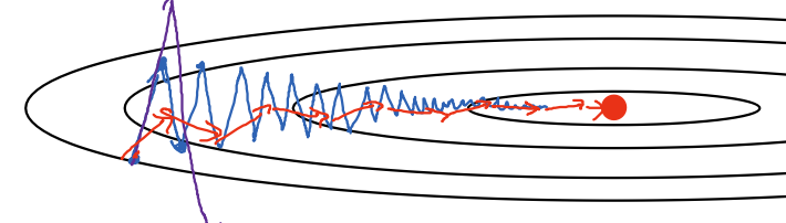
此时我们有两个Hyperparameter:$\alpha$和$\beta$,$\alpha$为learning rate,需要单独控制,$\beta$越大则梯度在水平方向下降幅度越大(stronger momentum),实际应用中,$\beta = 0.9$是一个很有效的经验值。
RMSprop
RMSprop(Root Mean Square prop)是另外一种加速梯度下降的优化,和上面的优化思路类似,RMSProp也是为了加快梯度在水平方向上下降的速度,减小梯度在垂直方向上的波动。其它的计算过程如下
- 对每个iteration $t$,计算当前mini-batch的$dw$和$db$
- 计算$S_{dw} = \beta S_{dw} + (1-\beta)S_{dw^2} \quad (dw^2 \quad \text {is element-wise square})$
- 计算$S_{db} = \beta S_{db} + (1-\beta)S_{db^2}$
- 跟新model的weights: $w := w - \alpha \frac{dw} {\sqrt {S_{dw} + \epsilon}} \quad (\epsilon = 10^{-8}) $
- 更新model的bias: $b := b - \alpha \frac{db} {\sqrt {S_{db} + \epsilon}} $
RMSProp和前面主要的不同点是,它是基于$dw$的平方来计算权重
Adam optimization algorithm
Adam(Adaptive moment estimation)优化算法是上述两种算法的结合,它的计算过程如下
- 初始化 $V_{dw} = 0$, $S_{dw} = 0, $$V_{db} = 0$, $S_{db} = 0$
- 对每个iteration $t$,计算当前mini-batch的$dw$和$db$
- 使用$\beta_1$计算momentum: $V_{dw} = \beta_1 V_{dw} + (1 - \beta_1) dw, \quad V_{db} = \beta_1 V_{db} + (1 - \beta_1) db$
- 使用$\beta_2$计算RMSProp: $S_{dw} = \beta_2 V_{dw} + (1 - \beta_2) dw^2, \quad S_{db} = \beta_2 V_{db} + (1 - \beta_2) db^2$
- 对$V$计算其bias correction: $V_{dw}^{\text{corrected}} = \frac{V_{dw}}{1 - \beta_1^t}, \quad V_{db}^{\text{corrected}} = \frac{V_{db}}{1 - \beta_1^t}$
- 对$S$计算其bias correction: $S_{dw}^{\text{corrected}} = \frac{S_{dw}}{1 - \beta_2^t}, \quad S_{db}^{\text{corrected}} = \frac{S_{db}}{1 - \beta_2^t}$
- 跟新model的weights: $w := w - \alpha \frac{V_{dw}^{\text{corrected}}} {\sqrt {S_{dw}^{\text{corrected}} + \epsilon}} $
- 更新model的bias: $b := b - \alpha \frac{V_{db}^{\text{corrected}}} {\sqrt {S_{db}^{\text{corrected}} + \epsilon}} $
几个Hyperparameters的参数取值如下
- $\alpha$: Learning rate需要仔细fine tune,没有固定数值
- $\beta_1$: 0.9,它影响 $dw$
- $\beta_2$: 0.999, 他影响 $dw^2$
- $\epsilon$: $10^{-8}$
Learning rate decay
另一种加速训练的方式是动态调整(逐步减小)learning rate,也叫做learning rate decay。在训练初期,我们可以用较大的$\alpha$,进行快速的梯度下降,当接近converge时,我们需要调整$\alpha$的值使步长变小,则可以帮助我们更快converge。动态调整$\alpha$的公式如下:
\[\alpha = \frac{1}{1 + \textit{decayRate} \times \textit{epochNumber}} \alpha_0\]假设$\alpha_0 = 0.2$, $decayRate = 1$,根据上面式子,随着epoch的增加,$\alpha$会逐步递减。
另一种控制$\alpha$的方式是使其在固定的时间间隔递减(例如每1000个epoch),这可以避免$\alpha$快速下降至0,如下图所示
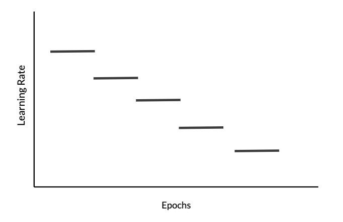
我们可以将 epoch 除以时间间隔$t$,其中$t$为恒定的窗口大小,其计算方式如下
\[\alpha = \frac{1}{1 + decayRate \times \lfloor\frac{epochNum}{timeInterval}\rfloor} \alpha_{0}\]其中 $\lfloor\frac{epochNum}{timeInterval}\rfloor$表示向下取整(numpy.floor)
def schedule_lr_decay(learning_rate0, epoch_num, decay_rate, time_interval=1000):
    learning_rate = 1 / (1 + decay_rate * np.floor(epoch_num/time_interval)) * learning_rate0
    return learning_rate
下面是一组使用learning rate decay的训练结果,可见随着时间的增加,$\alpha$在不断减小
| Epoch Number | Learning Rate | Cost |
|---|---|---|
| 0 | 0.100000 | 0.701091 |
| 1000 | 0.000100 | 0.661884 |
| 2000 | 0.000050 | 0.658620 |
| 3000 | 0.000033 | 0.656765 |
| 4000 | 0.000025 | 0.655486 |
| 5000 | 0.000020 | 0.654514 |
Resources
Appendix #1: Numpy implementation of Adam
def update_parameters_with_adam(parameters, grads, v, s, t, learning_rate = 0.01,
                                beta1 = 0.9, beta2 = 0.999,  epsilon = 1e-8):
    """
    Update parameters using Adam

    Arguments:
    parameters -- python dictionary containing your parameters:
                    parameters['W' + str(l)] = Wl
                    parameters['b' + str(l)] = bl
    grads -- python dictionary containing your gradients for each parameters:
                    grads['dW' + str(l)] = dWl
                    grads['db' + str(l)] = dbl
    v -- Adam variable, moving average of the first gradient, python dictionary
    s -- Adam variable, moving average of the squared gradient, python dictionary
    t -- Adam variable, counts the number of taken steps
    learning_rate -- the learning rate, scalar.
    beta1 -- Exponential decay hyperparameter for the first moment estimates
    beta2 -- Exponential decay hyperparameter for the second moment estimates
    epsilon -- hyperparameter preventing division by zero in Adam updates

    Returns:
    parameters -- python dictionary containing your updated parameters
    v -- Adam variable, moving average of the first gradient, python dictionary
    s -- Adam variable, moving average of the squared gradient, python dictionary
    """

    L = len(parameters) // 2                 # number of layers in the neural networks
    v_corrected = {}                         # Initializing first moment estimate, python dictionary
    s_corrected = {}                         # Initializing second moment estimate, python dictionary

    # Perform Adam update on all parameters
    for l in range(1, L + 1):
        # Moving average of the gradients. Inputs: "v, grads, beta1". Output: "v".
        v["dW" + str(l)] = beta1 * v["dW" + str(l)] + (1 - beta1) * grads['dW' + str(l)]
        v["db" + str(l)] = beta1 * v["db" + str(l)] + (1 - beta1) * grads['db' + str(l)]

        # Compute bias-corrected first moment estimate. Inputs: "v, beta1, t". Output: "v_corrected".
        v_corrected["dW" + str(l)] = v["dW" + str(l)] / (1 - np.power(beta1, t))
        v_corrected["db" + str(l)] = v["db" + str(l)] / (1 - np.power(beta1, t))

        # Moving average of the squared gradients. Inputs: "s, grads, beta2". Output: "s".
        s["dW" + str(l)] = beta2 * s["dW" + str(l)] + (1 - beta2) * np.power(grads['dW' + str(l)], 2)
        s["db" + str(l)] = beta2 * s["db" + str(l)] + (1 - beta2) * np.power(grads['db' + str(l)], 2)

        # Compute bias-corrected second raw moment estimate. Inputs: "s, beta2, t". Output: "s_corrected".
        s_corrected["dW" + str(l)] = s["dW" + str(l)] / (1 - np.power(beta2, t))
        s_corrected["db" + str(l)] = s["db" + str(l)] / (1 - np.power(beta2, t))

        # Update parameters. Inputs: "parameters, learning_rate, v_corrected, s_corrected, epsilon". Output: "parameters".
        parameters["W" + str(l)] -= learning_rate * v_corrected["dW" + str(l)] / (np.sqrt(s_corrected["dW" + str(l)]) + epsilon)
        parameters["b" + str(l)] -= learning_rate * v_corrected["db" + str(l)] / (np.sqrt(s_corrected["db" + str(l)]) + epsilon)

    return parameters, v, s, v_corrected, s_corrected