Recurrent Neural Network

Posted on 2018-05-14 | In AI , Machine Learning , Deep Learning

Sequence Data Notations

$x^{\langle i \rangle}$, 表示输入$x$中的第$i$个token
$y^{\langle i \rangle}$, 表示输出$y$中的第$i$个token
$x^{(i)\langle t \rangle}$，表示第$i$条输入样本中的第$t$个token
$y^{(i)\langle t \rangle}$，表示第$i$条输出样本中的第$t$个token
$n_x$，表示某个输入token向量长度
$n_y$，表示某个输出token长度
$x_5^{(2)\langle 3 \rangle\langle 4 \rangle}$, 表示第二条输入样本中，第三个layer中第4个token向量中的第五个元素

以文本输入为例，假设我们有一个10000个单词的字典和一串文本，现在的问题是，找出下面文本中是人名的单词，输出结果是一维向量，其中1代表名字

x: "Harry Potter and Hermione Granger invented a new spell."
y:  1 1 0 1 1 0 0 0 0

我们用$x^{\langle i \rangle}$表示上述句子中的每个单词，则$x^{\langle 1 \rangle}$表示Harry, $x^{\langle 2 \rangle}$表示Potter，以此类推。假设在我们的字典中，and这个单词排在第5位，则$x^{\langle 1 \rangle}$的值为一个一维向量

$x^{\langle 1 \rangle} = [0,0,0,0,1,0, ... ,0]$

注意上面的式子通常用列向量表示，即$x^{\langle i \rangle}$为[10000,1]。

在实际应用中，$x^{\langle 1 \rangle}$往往是一个2D tensor，因为我们通常一次输入$m$条训练样本(mini-batch)。我们假设m=20，则此时我们有20列向量，我们可以横向将它们stack成一个二维矩阵。比如上面例子中，RNN在某个时刻的输入tensor的大小是[10000,20]的。

相应的，上述句子对应的$y$表示如下，其中$y^{\langle i \rangle}$表示是名字的概率

$y = [1,1,0,1,1,0,0,0,0]$

Recurrent Neural Network

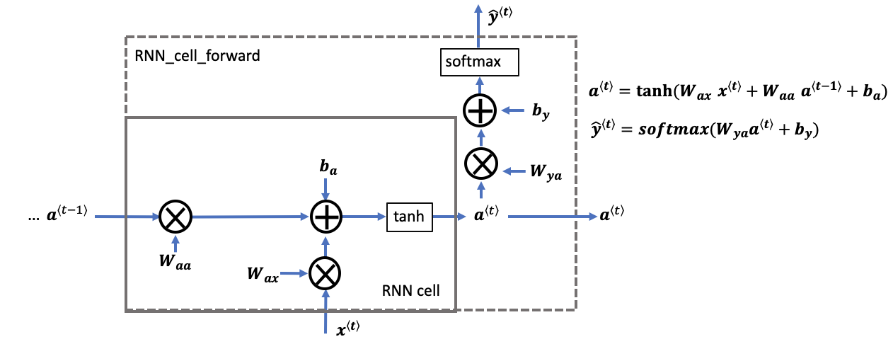
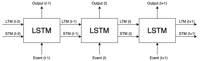
RNN的输入是一组sequence data，seguence中的每个$x^{\langle i \rangle}$会通过某一系列运算产生一个输出$y^{\langle i \rangle}$，并且该时间片上的输入除了有$x^{\langle i \rangle}$之外，还有可能来自前一个时间片的输出$a^{\langle i-1 \rangle}$，如下图所示

图中的$T$表示时间片，$a^{\langle {T_x} \rangle}$为$T$时刻的hidden state。我们令 $a^{\langle 0 \rangle} = 0$，则 $a^{\langle 1 \rangle}$ 和 $y^{\langle 1 \rangle}$的计算方式如下

$a^{\langle 1 \rangle} = g(W_{aa}a^{\langle 0 \rangle} + W_{ax}x^{\langle 1 \rangle} + b_a) \\ \hat y^{\langle 1 \rangle} = g(W_{ya}a^{\langle 1 \rangle} + b_y)$

对于$a^{\langle t \rangle}$, 其中常用的activation函数为$tanh$或$ReLU$，对于$\hat y^{\langle i \rangle}$，可以用$sigmoid$函数。Generalize一下

$a^{\langle t \rangle} = g(W_{aa}a^{\langle {t-1} \rangle} + W_{ax}x^{\langle t \rangle} + b_a) \\ \hat y^{\langle t \rangle} = g(W_y a^{\langle t \rangle} + b_y)$

简单起见，我们可以将$W_{aa}$和$W_{ax}$合并，假设，$W_{aa}$为[100,100], $W_{ax}$为[100,10000](通常来说$W_{ax}$较宽)，则可以将$W_{ax}$放到$W_{aa}$的右边，即$[W_{aa}|W_{ax}]$，则合成后的矩阵$W_{a}$为[100，10100]。$W_a$矩阵合并后，我们也需要将$a^{ \langle {t-1} \rangle}$和$x^{\langle t \rangle}$合并，合并方法类似，从水平改为竖直 $[\frac{a^{\langle {t-1} \rangle}}{x^{\langle t \rangle}}]$得到[10100,100]的矩阵。

$a^{\langle t \rangle} = g(W_a[a^{\langle {t-1} \rangle}, x^{\langle t \rangle}] + b_a) \\ \hat y^{\langle t \rangle} = g(W_y a^{\langle t \rangle} + b_y)$

因此，我们需要学习的参数便集中在了$W_a$, $b_a$和$W_y$,$b_y$上。在实际应用中，我们的$x$和$a$通常都是三维的矩阵

x.shape = (n_x, m, T_x)
a.shape = (n_a, m, T_a)

其中n_x表示x的one hot vector的长度(字典数量，比如5000)，m表示batch size，即样本数量(句子个数），T_x则表示每个样本的时间片数量（可以理解为句子中token的个数）。而$x^{(i)}$或者$a^{(i)}$为某个时刻t`的切片，即

x_i = x[:,:,t]
a_i = a[:,:,t]

Numpy的实现如下

def rnn_cell_forward(xt, a_prev, parameters):
    """
    Arguments:
    xt -- your input data at timestep "t", numpy array of shape (n_x, m).
    a_prev -- Hidden state at timestep "t-1", numpy array of shape (n_a, m)
    parameters -- python dictionary containing:
                        Wax -- Weight matrix multiplying the input, numpy array of shape (n_a, n_x)
                        Waa -- Weight matrix multiplying the hidden state, numpy array of shape (n_a, n_a)
                        Wya -- Weight matrix relating the hidden-state to the output, numpy array of shape (n_y, n_a)
                        ba --  Bias, numpy array of shape (n_a, 1)
                        by -- Bias relating the hidden-state to the output, numpy array of shape (n_y, 1)
    Returns:
    a_next -- next hidden state, of shape (n_a, m)
    yt_pred -- prediction at timestep "t", numpy array of shape (n_y, m)
    cache -- tuple of values needed for the backward pass, contains (a_next, a_prev, xt, parameters)
    """
    
    # Retrieve parameters from "parameters"
    Wax = parameters["Wax"]
    Waa = parameters["Waa"]
    Wya = parameters["Wya"]
    ba = parameters["ba"]
    by = parameters["by"]
    
    # compute next activation state using the formula given above
    a_next = np.tanh(np.dot(Wax, xt) + np.dot(Waa, a_prev) + ba)
    # compute output of the current cell using the formula given above
    yt_pred = softmax(np.dot(Wya, a_next) + by)
    # store values you need for backward propagation in cache
    cache = (a_next, a_prev, xt, parameters)
    
    return a_next, yt_pred, cache

def rnn_forward(x, a0, parameters):
    """
    Arguments:
    x -- Input data for every time-step, of shape (n_x, m, T_x).
    a0 -- Initial hidden state, of shape (n_a, m)
    parameters -- python dictionary containing:
                        Waa -- Weight matrix multiplying the hidden state, numpy array of shape (n_a, n_a)
                        Wax -- Weight matrix multiplying the input, numpy array of shape (n_a, n_x)
                        Wya -- Weight matrix relating the hidden-state to the output, numpy array of shape (n_y, n_a)
                        ba --  Bias numpy array of shape (n_a, 1)
                        by -- Bias relating the hidden-state to the output, numpy array of shape (n_y, 1)

    Returns:
    a -- Hidden states for every time-step, numpy array of shape (n_a, m, T_x)
    y_pred -- Predictions for every time-step, numpy array of shape (n_y, m, T_x)
    caches -- tuple of values needed for the backward pass, contains (list of caches, x)
    """
    
    # Initialize "caches" which will contain the list of all caches
    caches = []
    
    # Retrieve dimensions from shapes of x and parameters["Wya"]
    n_x, m, T_x = x.shape
    n_y, n_a = parameters["Wya"].shape
    
    a = np.zeros((n_a, m, T_x))
    y_pred = np.zeros((n_y, m, T_x))

    a_next = a0
    
    # loop over all time-steps
    for t in range(T_x):
        # Update next hidden state, compute the prediction, get the cache
        a_next, yt_pred, cache = rnn_cell_forward(x[:,:,t], a_next, parameters)
        # Save the value of the new "next" hidden state in a
        a[:,:,t] = a_next
        # Save the value of the prediction in y
        y_pred[:,:,t] = yt_pred
        # Append "cache" to "caches"
        caches.append(cache)
    
    # store values needed for backward propagation in cache
    caches = (caches, x)
    
    return a, y_pred, caches

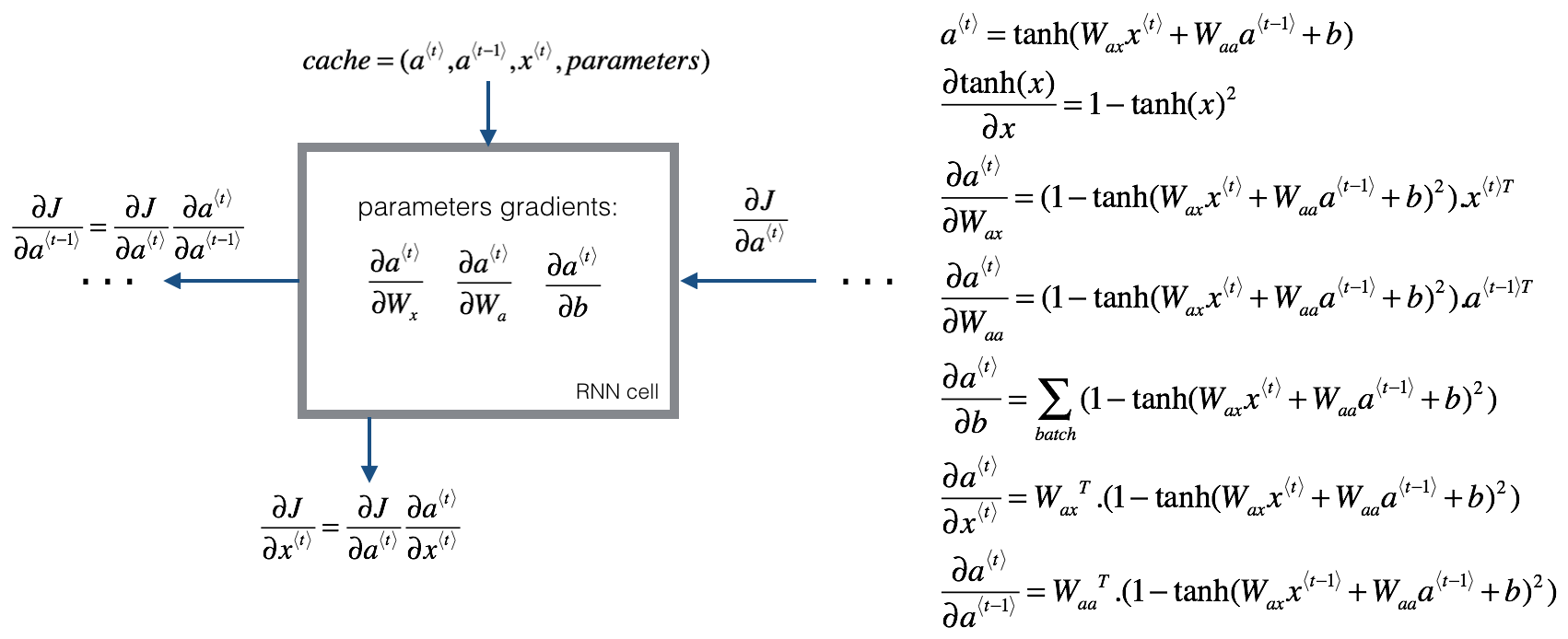
Loss函数

上一节中我们已经看到，对每条训练样本来说，任何一个单词产生的输出$\hat y^{(i)\langle t \rangle}$是一个一维向量，形式和分类问题类似，因此对于单个单词的loss函数可以用逻辑回归的loss函数

$L^{\langle t \rangle}(\hat y ^{\langle t \rangle}, y^{\langle t \rangle}) = - y^{\langle t \rangle}log{y^{\langle t \rangle}} - (1-y^{\langle t \rangle})log{(1-y^{\langle t \rangle})}$

则对于整个样本（句子），loss函数为每个单词loss的和

$L(\hat y, y) = \sum_{t=1}^{T} L^{\langle t \rangle}(\hat y ^{\langle t \rangle}, y^{\langle t \rangle})$

反向求导的过程如下

不同的RNN网络

除了上面提到的一种RNN网络外，根据实际应用的不同，RNN可以衍生出不同的结构，如下图所示

Language Model

Language Model有很多种，其输入为一个句子，输出为预测结果，通常以概率形式表示。假如我们的字典有10000个单词，输入文本如下

Cats average 15 hours of sleep a day. <EOS>

我们可以参考前面提到的RNN网络来构建我们的Model，如下图所示

其中每个cell的结构如下图所示

另$x^{\langle 1 \rangle}$和$a^{\langle 0 \rangle}$均为0，输出$\hat y^{\langle 1 \rangle}$是一个softmax结果，表示字典中每个单词出现的概率，是一个[10000,1]的向量，由于未经训练，每个单词出现的概率均为1/10000
接下来我们用真实$y^{\langle 1 \rangle}$（”Cats”在字典中出现的概率）和 $a^{\langle 1 \rangle}$作为下一层的输入，得到$\hat y^{\langle 2 \rangle}$，其含义为当给定前一个单词为”Cats”时，当前单词是字典中各个单词的概率即 $P(?? |Cats)$，因此$\hat y^{\langle 2 \rangle}$也是[10000,1]的。注意到，此时的$x^{\langle 2 \rangle} = y^{\langle 1 \rangle}$
类似的，第三层的输入为真实结果$y^{\langle 2 \rangle}$，即$P(average |Cats)$，和$a^{\langle 2 \rangle}$，输出为$\hat y^{\langle 2 \rangle}$，表示$P(?? |Cats average)$。同理，此时$x^{\langle 3 \rangle} = y^{\langle 2 \rangle}$
重复上述步骤，直到走到EOS的位置

上述的RNN模型可以做到根据前面已有的单词来预测下一个单词是什么

梯度消失

不难发现，上面的RNN模型是基于前面的单词来预测后面出现的单词出现的概率，但是对于一些长句子，单词前后的联系可能被分隔开，比如英语中的定语从句

The cat, which already ate ... , was full
The cats, which already ate ..., were full

上面例子例子中cat和was, cats和were中间隔了一个很长的定语修饰，这就会导致当RNN在预测was或者were时，由于前面的主语信息(cat或者cats)位置很靠前，使得预测概率受到影响（如果RNN能识别出此时主语是cat/cats则was/were的预测概略应该会提高）。具体在RNN中的表现是当做back prop时，由于网络太深，会出现梯度消失的问题，也就是说我们无法通过back prop来影响到cat后者cats的weight。

GRU

GRU(Gated Recurrent Uinit)被设计用来解决上述问题，其核心思想是为每个token引入一个GRU unit - $c^{\langle t \rangle}$，计算方式如下

$\hat c^{\langle t \rangle} = tanh (W_c[c^{\langle {t-1} \rangle}, x^{\langle t \rangle}] + b_c) \\ \Gamma_u ^{\langle t \rangle} = \delta (W_u[c^{\langle {t-1} \rangle}, x^{\langle t \rangle}] + b_u) \\ c^{\langle t \rangle} = \Gamma_u ^{\langle t \rangle} * \hat c^{\langle t \rangle} + (1-\Gamma_u ^{\langle t \rangle}) * c^{\langle {t-1} \rangle}$

其中，$\Gamma_u ^{\langle t \rangle}$用来控制是否更新$c^{\langle t \rangle}$的值，$\delta$通常为sigmoid函数，因此$\Gamma_u ^{\langle t \rangle}$的取值为0或1；*为element-wise的乘法运算

回到上面的例子，假设我们cats对应的$c^{\langle t \rangle}$值为0或1, 1表示主语是单数，0表示主语是复数。则直到计算was/were之前，$c^{\langle t \rangle}$的值会一直被保留，作为计算时的参考，保留的方式则是通过控制$\Gamma_u ^{\langle t \rangle}$来完成

Tha cat,    which   already   ate ...,   was    full.
    c[t]=1                               c[t]=1
    g[t]=1  g[t]=0  g[t]=0    g[t]=0 ... g[t]=0  

可以看到当$\Gamma_u ^{\langle t \rangle} $为1时，$c^{\langle t \rangle} = c^{\langle {t-1} \rangle} = a^{\langle {t-1} \rangle}$，则前面的信息可以被一直保留下来。

注意到$c^{\langle t \rangle}, \hat c^{\langle t \rangle}, \Gamma_u ^{\langle t \rangle}$均为向量，其中$\Gamma_u ^{\langle t \rangle}$向量中的值为0或1，则上面最后一个式子的乘法计算为element-wise的，这样$\Gamma_u ^{\langle t \rangle}$就可以起到gate的作用。

LSTM

Long Short Term Memory(LSTM)是另一种通过建立前后token链接来解决梯度消失问题的方法，相比GRU更为流行一些。和GRU不同的是

LSTM使用$a^{\langle {t-1} \rangle}$来计算 $\hat c^{\langle t \rangle}$和$\Gamma_u ^{\langle t \rangle}$
LSTM使用两个gate来控制$c^{\langle t \rangle}$，一个前面提到的$\Gamma_u ^{\langle t \rangle}$，另一个是forget gate - $\Gamma_f ^{\langle t \rangle}$
LSTM使用了一个output gate来控制$a^{\langle t \rangle}$

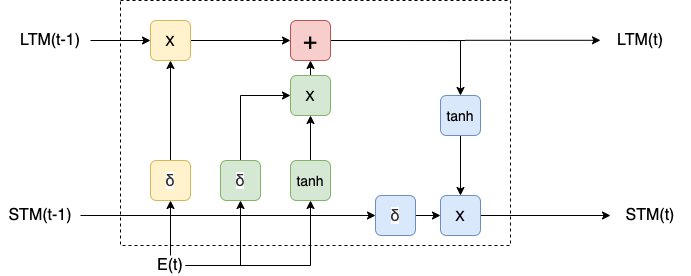
$\hat c^{\langle t \rangle} = tanh (W_c[a^{\langle {t-1} \rangle}, x^{\langle t \rangle}] + b_c) \\ \Gamma_u ^{\langle t \rangle} = \delta (W_u[a^{\langle {t-1} \rangle}, x^{\langle t \rangle}] + b_u) \\ \Gamma_f ^{\langle t \rangle} = \delta (W_f[a^{\langle {t-1} \rangle}, x^{\langle t \rangle}] + b_f) \\ c^{\langle t \rangle} = \Gamma_u ^{\langle t \rangle} * \hat c^{\langle t \rangle} + \Gamma_f ^{\langle t \rangle} * c^{\langle {t-1} \rangle} \\ \Gamma_o ^{\langle t \rangle} = \delta (W_o[a^{\langle {t-1} \rangle}, x^{\langle t \rangle}] + b_o) \\ a^{\langle t \rangle} = \Gamma_o * tanh(c^{\langle t \rangle})$

上述LSTM式子引入了三个gate函数，虽然步骤比较复杂，但是逻辑上还是比较清晰，也容易更好的整合到RNN网络中，下图是一个引入了LSTM的RNN的计算单元

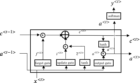
每个LSTM单元都是可微分的，它里面一共包含四种运算：加法，乘法，tanh和 sigmoid每种运算均可微。如果把各个LSTM单元串联起来，则RNN的模型变为

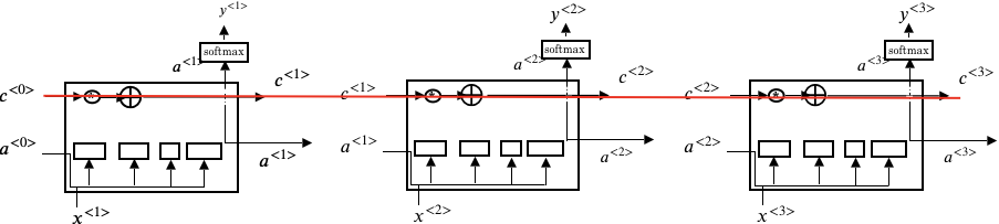
上述红线表示了$c^{\langle t \rangle}$的记忆过程，通过gate的控制，可以使$c^{\langle 3 \rangle} = c^{\langle 1 \rangle}$, 从而达到缓存前面信息的作用，进而可以解决梯度消失的问题。

另一种更加直观理解LSTM的方式是LSTM cell看成四个gate的组合

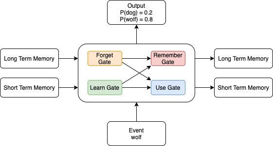
将每个RNN cell串联起来可已得到

Learn Gate

Learn Gate首先将short-term memroy($STM_{(t-1)}$)和$E_t$进行combine，然后将结果和一个ignore vector进行element-wise的相乘来决定矩阵中那些元素需要保留，哪些舍弃。这个ignore vector同样是通过$STM_{(t-1)}$和$E_t$生成，只是非线性函数用了sigmoid来限制输出的值域。

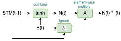
其中$N_t$和$i_t$表示为

$N_t = tanh(W_n{[STM_{t-1}, E_t]}+b_n) \\ i_t = \delta(W_i{[STM_{t-1}, E_t]}+b_i)$

Forget Gate

Forget Gate用来控制long-term memory中哪些保留哪些舍弃，具体做法是$LTM_{t-1}$乘以一个forget factor$f(t)$。

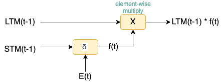
其中$f(t)$计算如下

$f(t) = \delta(W_f{[STM_{t-1}, E_t]}+b_f)$

Remember Gate

Remember Gate将上面两个gate的输出进行相加

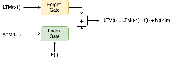
Use Gate

Use Gate的输入来自Learn Gate和Forget Gate，组合方式如下

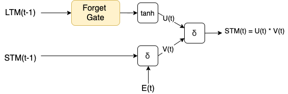
其中$U_t$和$V_t$的计算方式如下

$U_t = tanh(W_uLTM_{t-1}f_t + b_u) \\ V_t = \delta(W_v[STM_{t-1}, E_t] + b_v)$

我们将上面四个gate组合到一起，可以得到下面的结果，和我们上面的结构类似

LSTM的numpy实现

def lstm_cell_forward(xt, a_prev, c_prev, parameters):
    """
    Arguments:
    xt -- your input data at timestep "t", numpy array of shape (n_x, m).
    a_prev -- Hidden state at timestep "t-1", numpy array of shape (n_a, m)
    c_prev -- Memory state at timestep "t-1", numpy array of shape (n_a, m)
    parameters -- python dictionary containing:
                        Wf -- Weight matrix of the forget gate, numpy array of shape (n_a, n_a + n_x)
                        bf -- Bias of the forget gate, numpy array of shape (n_a, 1)
                        Wi -- Weight matrix of the update gate, numpy array of shape (n_a, n_a + n_x)
                        bi -- Bias of the update gate, numpy array of shape (n_a, 1)
                        Wc -- Weight matrix of the first "tanh", numpy array of shape (n_a, n_a + n_x)
                        bc --  Bias of the first "tanh", numpy array of shape (n_a, 1)
                        Wo -- Weight matrix of the output gate, numpy array of shape (n_a, n_a + n_x)
                        bo --  Bias of the output gate, numpy array of shape (n_a, 1)
                        Wy -- Weight matrix relating the hidden-state to the output, numpy array of shape (n_y, n_a)
                        by -- Bias relating the hidden-state to the output, numpy array of shape (n_y, 1)
                        
    Returns:
    a_next -- next hidden state, of shape (n_a, m)
    c_next -- next memory state, of shape (n_a, m)
    yt_pred -- prediction at timestep "t", numpy array of shape (n_y, m)
    cache -- tuple of values needed for the backward pass, contains (a_next, c_next, a_prev, c_prev, xt, parameters)
    
    Note: ft/it/ot stand for the forget/update/output gates, cct stands for the candidate value (c tilde),
          c stands for the cell state (memory)
    """

    # Retrieve parameters from "parameters"
    Wf = parameters["Wf"] # forget gate weight
    bf = parameters["bf"]
    Wi = parameters["Wi"] # update gate weight (notice the variable name)
    bi = parameters["bi"] # (notice the variable name)
    Wc = parameters["Wc"] # candidate value weight
    bc = parameters["bc"]
    Wo = parameters["Wo"] # output gate weight
    bo = parameters["bo"]
    Wy = parameters["Wy"] # prediction weight
    by = parameters["by"]
    
    # Retrieve dimensions from shapes of xt and Wy
    n_x, m = xt.shape
    n_y, n_a = Wy.shape

    concat = np.zeros((n_a + n_x, m))
    concat[: n_a, :] = a_prev
    concat[n_a :, :] = xt

    # Compute values for ft, it, cct, c_next, ot, a_next
    ft = sigmoid(np.dot(Wf, concat) + bf)
    it = sigmoid(np.dot(Wi, concat) + bi)
    cct = np.tanh(np.dot(Wc, concat) + bc)
    c_next = ft * c_prev + it * cct
    ot = sigmoid(np.dot(Wo, concat) + bo)
    a_next = ot * np.tanh(c_next)
    
    # Compute prediction of the LSTM cell
    yt_pred = softmax(np.dot(Wy, a_next) + by)

    # store values needed for backward propagation in cache
    cache = (a_next, c_next, a_prev, c_prev, ft, it, cct, ot, xt, parameters)

    return a_next, c_next, yt_pred, cache

def lstm_forward(x, a0, parameters):
    """
    Arguments:
    x -- Input data for every time-step, of shape (n_x, m, T_x).
    a0 -- Initial hidden state, of shape (n_a, m)
    parameters -- python dictionary containing:
                        Wf -- Weight matrix of the forget gate, numpy array of shape (n_a, n_a + n_x)
                        bf -- Bias of the forget gate, numpy array of shape (n_a, 1)
                        Wi -- Weight matrix of the update gate, numpy array of shape (n_a, n_a + n_x)
                        bi -- Bias of the update gate, numpy array of shape (n_a, 1)
                        Wc -- Weight matrix of the first "tanh", numpy array of shape (n_a, n_a + n_x)
                        bc -- Bias of the first "tanh", numpy array of shape (n_a, 1)
                        Wo -- Weight matrix of the output gate, numpy array of shape (n_a, n_a + n_x)
                        bo -- Bias of the output gate, numpy array of shape (n_a, 1)
                        Wy -- Weight matrix relating the hidden-state to the output, numpy array of shape (n_y, n_a)
                        by -- Bias relating the hidden-state to the output, numpy array of shape (n_y, 1)
                        
    Returns:
    a -- Hidden states for every time-step, numpy array of shape (n_a, m, T_x)
    y -- Predictions for every time-step, numpy array of shape (n_y, m, T_x)
    c -- The value of the cell state, numpy array of shape (n_a, m, T_x)
    caches -- tuple of values needed for the backward pass, contains (list of all the caches, x)
    """

    # Initialize "caches", which will track the list of all the caches
    caches = []
    
    ### START CODE HERE ###
    Wy = parameters['Wy'] # saving parameters['Wy'] in a local variable in case students use Wy instead of parameters['Wy']
    # Retrieve dimensions from shapes of x and parameters['Wy']
    n_x, m, T_x = x.shape
    n_y, n_a = parameters["Wy"].shape
    
    # initialize "a", "c" and "y" with zeros
    a = np.zeros((n_a, m, T_x))
    c = np.zeros((n_a, m, T_x))
    y = np.zeros((n_y, m, T_x))
    
    # Initialize a_next and c_next
    a_next = a0
    c_next = np.zeros(a_next.shape)
    
    # loop over all time-steps
    for t in range(T_x):
        # Get the 2D slice 'xt' from the 3D input 'x' at time step 't'
        xt = x[:,:,t]
        # Update next hidden state, next memory state, compute the prediction, get the cache
        a_next, c_next, yt, cache = lstm_cell_forward(x[:, :, t], a_next, c_next, parameters)
        # Save the value of the new "next" hidden state in a
        a[:,:,t] = a_next
        # Save the value of the next cell state
        c[:,:,t]  = c_next
        # Save the value of the prediction in y
        y[:,:,t] = yt
        # Append the cache into cache
        caches.append(cache)
        
    
    # store values needed for backward propagation in cache
    caches = (caches, x)

    return a, y, c, caches

Recurrent Neural Network

Sequence Data Notations

Recurrent Neural Network

Loss函数

不同的RNN网络

Language Model

梯度消失

GRU

LSTM

Resources