Word Embeddings

Word Embeddings

之前我们将输入文本用一个 1 hot vector 来表示，它是建立在一个 dictionary 的基础上，比如单词cat的表示方式为

[0, 0, 0, ..., 1, ..., 0, 0]

1表示其在 dictionary 中的 index，我们用$O_{index}$表示。上面例子中，cat在字典中的 index 为 5791，则对应的表示为${O_{5791}}$。

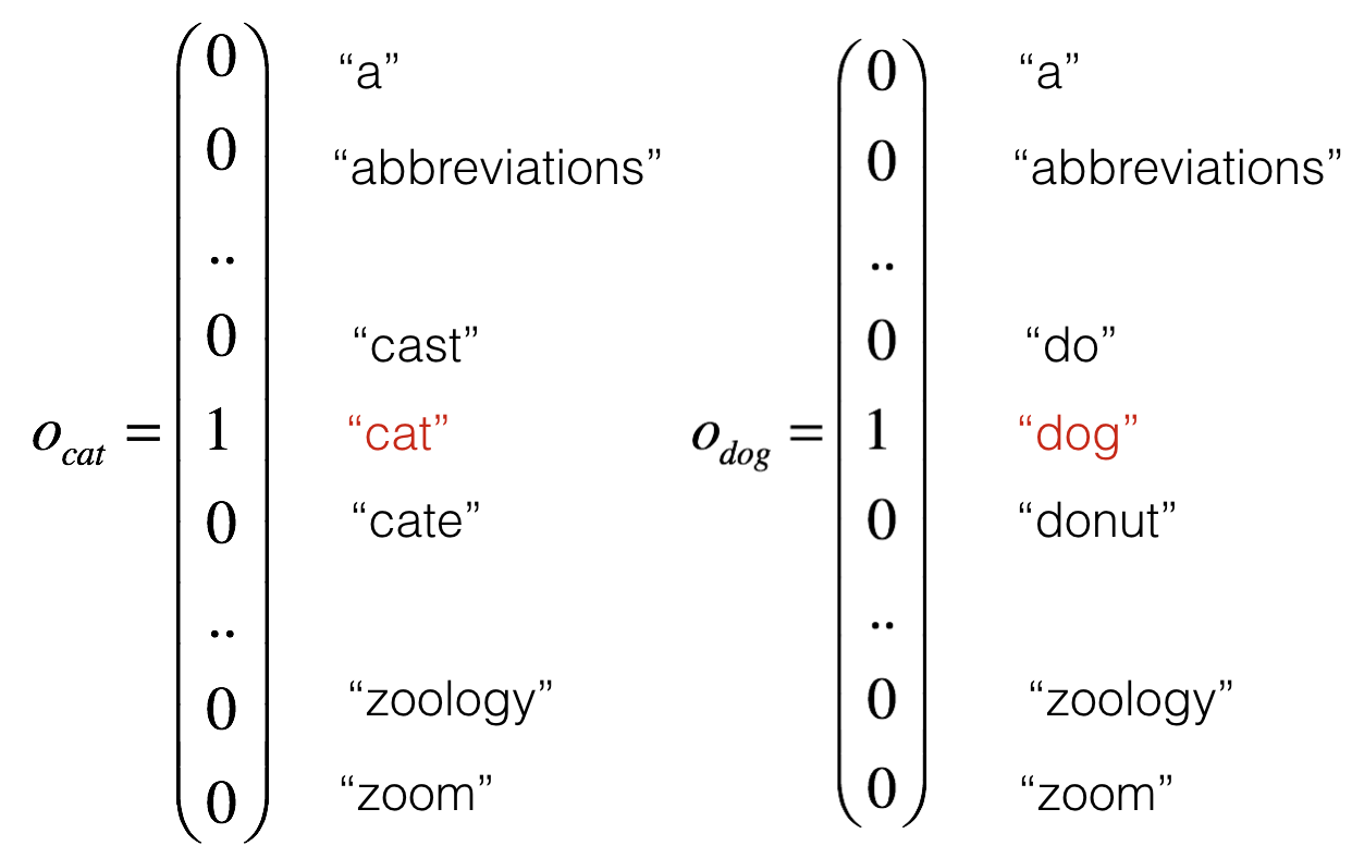
不难发现，对任意两个不同的 word，他们所对应向量之间的 inner product 为0。这说明 word 之间完全正交，即使他们有相关性，系统也无法 generalize，例如

I want a glass of orange juice
I want a glass of apple ____

即使系统可以推测出orange juice，但是当下次遇到 apple时，由于apple和orange正交，则之前的结果无法 generalize 到 apple 上面，此时还需要计算得到 apple juice，效率非常低。因此我们可以换一种形式来表示一个 word。

我们可以给字典里的每个 word 关联一些 feature，比如

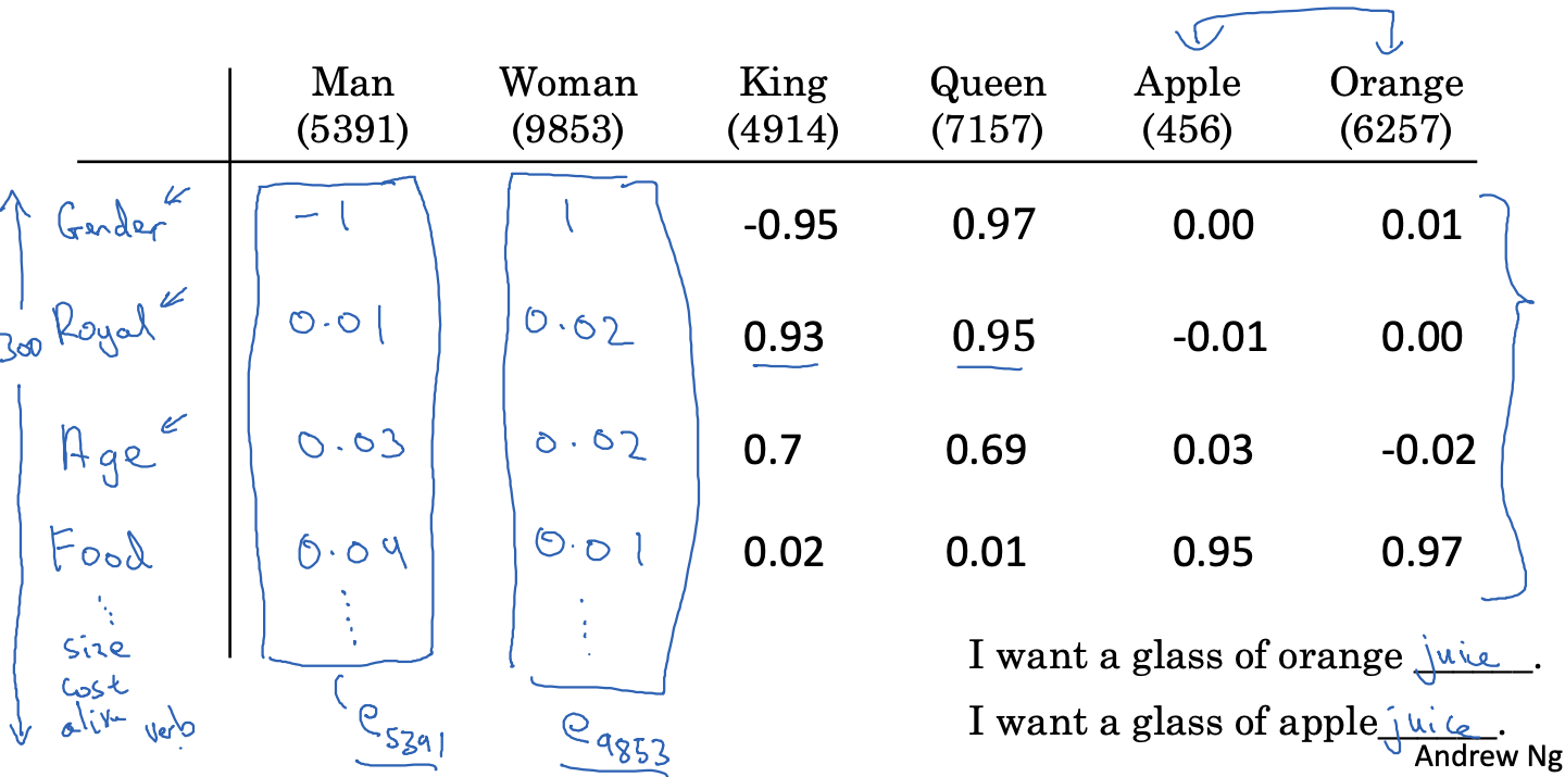
图中我们为每个 word 关联了 300 个 feature，因此每个 word 可以用一个[300, 1]的 vector 表示，对于单词Man所对应的 vector，我们用 $e_{5391}$ 来表示。这样两个相似的 word，他们的 feature vector 也是相似的，比如Apple和Orange。

回到最开始 RNN 的那个例子，假设我们有一个句子，我们需要识别出那些 word 是人名

x = ["Sally", "Johnson", "is", "an", "orange", "farmer"]
y = [1, 1, 0, 0, 0, 0]

之前每个 word 使用 1 hot vector 来表示，现在则可以用 word embedding 来表示。那么 word embedding 从哪里来呢？我们需要自己训练 model 来得到每个 word 的 embedding。另一种方式是下载已经训练好的embedding model。对于每个 word 来说，我们可以想象将其 encode 成一个 vector，vector中的每个值代表一个描述这个词的feature或者一个单独的dimenson。embedding就是这些vector的集合。

在实际应用中，我们可以用一个很大的 unlabeled text 数据集来 train 我们的 embedding model，然后在 transfer learning 到一个 small dataset 上面:

1. Learn word embeddings from a large text corpus (1-100B words), or download a pre-trained embedding online
2. Transfer embedding to new task with smaller training set (say, 100k words)
3. Optional: Continue to fine tune the word embeddings with new data.

回到前面说的相关性问题，当我们将word映射成embedding vector之后，我们如何来描述各个vector之间的相关性呢？一种方法是使用 Cosine Similarity，即给定两个vector $u$和$v$，计算下面式子

Cosine Similarity 的值取决于$u$, $v$之间的夹角。如果$u$, $v$相似度越高，那么它们之间的夹角越趋向于0(cosine值趋向于1)，反之，则夹角趋向于90甚至180度

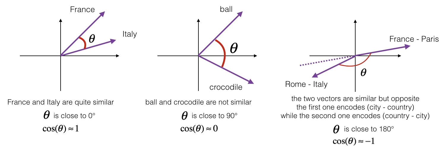
Appendix #1 展示了如何用Python计算两个vector的相似度。除了使用余弦相似度以外，也可以使用L2范数(欧几里得距离)，这里不展开讨论

由之前的Computer Graphic文章可知，Cosine Similarity的代数表达为两个vector的点积(Dot Product)。因此，我们通常用点积来描述两个embedding vector在 多维空间的相似度，如果点积的值越大，则表示它们在语义上越接近，反之则越疏远，这点和cosine的表达是类似的。

Embedding Matrix

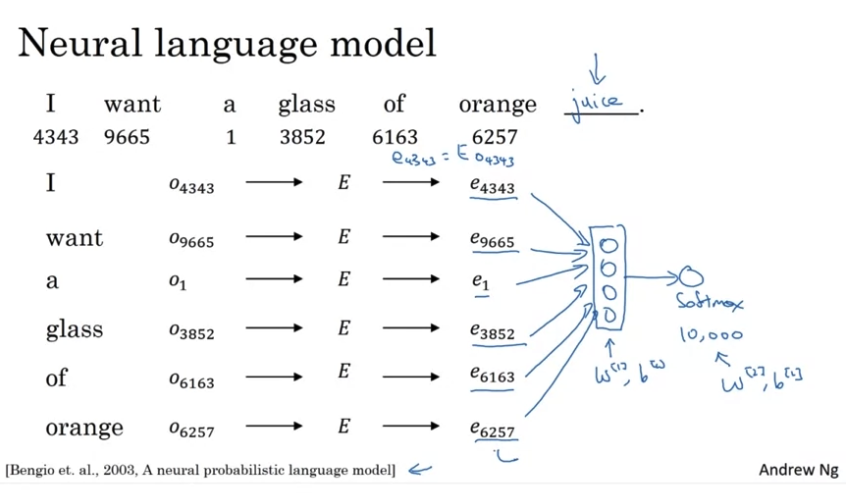
假设我们的字典有10,000个单词，每个单词的 feature vector 是[300, 1]，那么整个 embedding matrix 为[300, 10,000]，每一个列向量代表一个词所有的 feature，我们的目标就是 train 我们的 network 来找到这个 embedding matrix

如果我们用这个 embedding matrix E (300, 10,000) 去和一个 one-hot vector O(10,000, 1)相乘，结果是一个(300, 1)的 vector e

Word2Vec

Word2Vec 是一种相对比较高效的 learn word embedding 的一种算法。它的大概意思，选取一个 context word，比如”orange” 和一个 target word 比如 “juice”，我们通过构建 neural network 找到将 context word 映射成 target word 的 embedding matrix。通常来说，这个 target word 是 context word 附近的一个 word，可以是 context word 向前或者向后 skip 若干个 random word 之后得到的 word。

如果从 model 的角度来来说，它的 input 是一个 word，output 是它周围的一个 context word。

还是假定我们的字典大小为10,000，每个 feature vector 的 dim 是300，那么 embedding 的 matrix 大小为[10,000, 300]，我们的输入用 word 的 1-hot vector 表示，即是一个[10,000, 1]的稀疏向量，则我们 model 定义如下

# for each input word, predict its context words surrounding it
class SkipGram(nn.Module):
    def __init__(self, n_vocab, n_embed):
        super().__init__()

        # complete this SkipGram model
        self.embedding = nn.Embedding(n_vocab, n_embed)
        self.fc = nn.Linear(n_embed, n_vocab)
        self.softmax = nn.LogSoftmax(dim=1)

    def forward(self, x):
        x = self.embedding(x)
        x = self.fc(x)
        x = self.softmax(x)
        return x

nn.Embedding

Negative Sampling

上面的SkipGram有一个性能问题是如果字典数量过大会导致 softmax 方法非常耗时。这里介绍另一种相对高效的 network，叫做 Negtive Sampling。它的大概意思是，给一组 context word 和 target word，判断他们是否是符合语义，比如

x1: (orange, juice), y1:1
x2: (orange, king), y2:0

选取这个 pair 的方式和上面一样，sample 一下 context word，然后随机选取某一个 context word 周围一个 word(window 可以是左右 10 个 word 以内)作为 target word。

因此，我们 model 变成了一个 logistic regression model，它的 input 是一个 pair，output 是0或1用来表示这个 pair 是否正确。

context_embed = nn.Embedding(n_vocab, n_embed)
target_embed = nn.Embedding(n_vocab, n_embed)

P(y=1 | c,t) = sigmoid(target_embed.t() * context_embed)

当我们 train 这个 model 的时候，我们的 training dataset 需要有 negative examples:

context |  word | target?
--------------------------
orange  | juice | 1
range   | king  | 0
orange  | book  | 0
orange  | the   | 0
orange  | of    | 0

但实际上我们 train 的时候，y不需要包含 10,000 个结果，而只需要K个，其中K-1个为 negative example，K可以为 4

Resources

• The Unreasonable Effectiveness of Recurrent Neural Networks
• Deep Learning Specialization Course on Coursera
• Deep Learning with PyTorch

Appendix #1: cosine_similarity

def cosine_similarity(u, v):
    """
    Cosine similarity reflects the degree of similarity between u and v
        
    Arguments:
        u -- a word vector of shape (n,)          
        v -- a word vector of shape (n,)

    Returns:
        cosine_similarity -- the cosine similarity between u and v defined by the formula above.
    """    
    # Special case. Consider the case u = [0, 0], v=[0, 0]
    if np.all(u == v):
        return 1

    dot = np.sum(u*v) 
    # Compute the L2 norm of u 
    norm_u = np.sqrt(np.sum(u**2))    
    # Compute the L2 norm of v (≈1 line)
    norm_v = np.sqrt(np.sum(v**2))
    
    # Avoid division by 0
    if np.isclose(norm_u * norm_v, 0, atol=1e-32):
        return 0
    
    # Compute the cosine similarity defined by formula
    cosine_similarity = dot/(norm_u * norm_v)
    
    return cosine_similarity

def cosine_similarity_test():
    father = word_to_vec_map["father"]
    mother = word_to_vec_map["mother"]
    ball = word_to_vec_map["ball"]
    crocodile = word_to_vec_map["crocodile"]
    france = word_to_vec_map["france"]
    italy = word_to_vec_map["italy"]
    paris = word_to_vec_map["paris"]
    rome = word_to_vec_map["rome"]

    cosine_similarity(father, mother) # 0.8909038442893616
    cosine_similarity(ball, crocodile) # 0.2743924626137942
    cosine_similarity(france - paris, rome - italy) # -0.6751479308174201