Sequence Models and Attention Mechanism

Basic Models

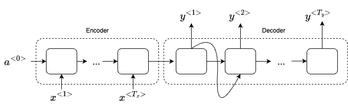
Let’s say you want to input a French sentence like Jane visite I'Afrique Septembre, and you want to translate it to the English sentence, Jane is visiting Africa in September. How can you train a neural network to input the sequence x and output the sequence y?

First, let’s build a LSTM as an encoder network. We feed the network with one word a time from the original french sentence. After ingesting the input sequence the RNN then outputs a vector that represents the input sentence. After that, we can build a decoder network that takes the input from the encoder and outputs the translated English words.

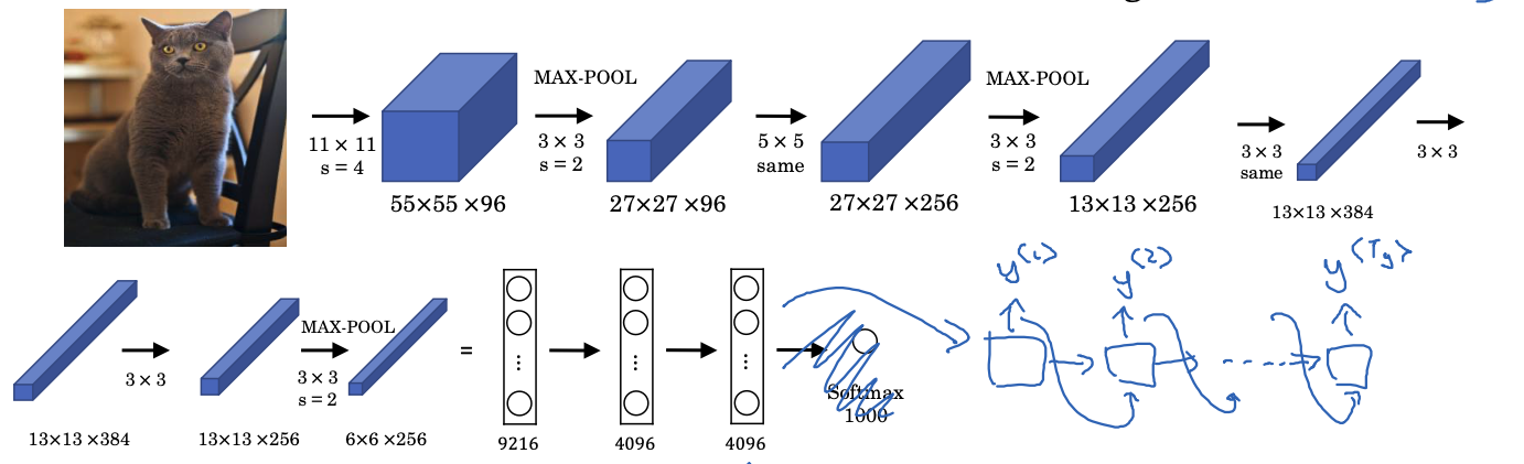
Similarly, we can use the same encoder and decoder architecture for image captioning. Our encoder will be a CNN model (e.g., AlexNet), and we replace the last layer (softmax) with an RNN decoder. This model works quite well especially for generating text that are not so long.

Machine translation as building a conditional language model

Since the decoder in a machine translation model is an RNN, it generates text probabilistically, meaning it can produce multiple translations for the same English sentence:

 Jane visite I'Afrique Septembre 

-> Jane is visiting Africa in September.
-> Jane is going to be visiting Africa in September.
-> In September, Jane will visit Africa.
-> Her African friend welcomed Jane in September.

However, we don’t want to output a random English translation, we want to output the best and the most likely English translation. In the example above, clearly, the first translation is the most accurate, while the others are suboptimal.

But how can we control this generation process? We can frame it as a conditional probability problem: given an input $x$, we aim to compute the probability of a sequence $y^{t}$:

A naive approach is greedy search, where at each step, we select the word $y^{t}$ with the highest probability. However, this strategy often fails to produce the best overall translation because it optimizes for immediate word probabilities at each step rather than considering the global sequence structure. In this case, the probability of choosing Jane is going to is higher than Jane is visiting, as going is a more commonly seen word in English.

Instead, what we need to do, is to find a search algorithm that can find the following value for us:

Beam Search Algorithm

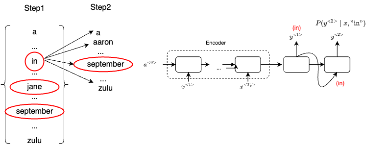
Let’s explain the Beam Search algorithm using our running example above. Once our decoder outputs the probability of the first English word (the outputs are from a softmax layer that contains the possibility over 1000 words), represented as $P(y^{<1>} \mid x)$, unlike greedy search, Beam will consider multiple candidates. The number of candidates is set by beam width. If beam_width = 3, then Beam will look at three candidates at a time.

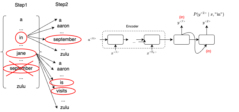
Let’s say when evaluating the first words, it finds that the choices "in", "jane" and "september" are the most likely three possibilities for English outputs. Then Beam search will save the words in memory that it wants to try all three of these words.

For each of these three choices consider what should be the second word, so after "in", maybe a second word is "a","aaron", "september" or "zulu". To evaluate the probability of second word $y^{<2>}$, we will use our decoder network fragments where the input from the previous block is $y^{<1>}$ ("in").

By hard-wiring $y^{<1>}$ one, we evaluate the probability of the second word given the first word of the translation has been the word “in” - $P(y^{<2>} \mid x, \text {“in”})$

Note that the goal of the second step of beam search is to find the pair of the first and second words that is most likely, not just a second where is most likely.

We repeat the same from process to calculate the most likely second words for "jane" and "september". Let’s say we have 10,000 words in the dictionary. In step 2, with the beam width equals to 3, we will need to evaluate 3 x 10000 options (10000 for each word). We then pick the top 3 most likely words based on the evaluation result from the above formula (the one with the highest conditional probability wins).

For example, in step 2, the "september" is most likely to picked after "in". And for "jane", the model picks "is" and "visits". Note that since beam_width = 3, and we already picked three words, that means "september" will be skipped.

For step 3, we simply repeat the same process above. The three words are "in september", "jane is" and "jane visits", as shown below:

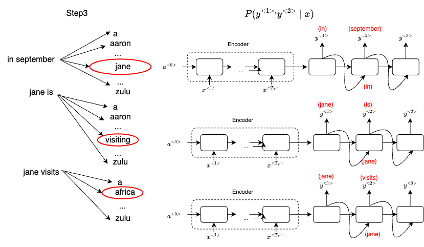
And the final outcome of this process will be that adding one word at a time that Beam search will decide that "Jane visits Africa in September. <EOS>" will be terminated by the end of sentence symbol.

Refinements to Beam Search

Notice that the formula we use to determine the most likely words is the product of a sequence of probability numbers

Note that these probabilities are all numbers less than one, and multiplying a lot of these numbers result in a tiny number, which can result in numerical under-floor, meaning that is too small for the floating point of representation in your computer to store accurately.

In practice, instead of maximizing this product, we will take logs:

Then a log of a product becomes a sum of log, and maximizing this sum of log probabilities should give you the same results in terms of selecting the most likely sentence. We can further improve the formula to be more computing efficient

Instead of calculating the argmax of the log product, we normalize the value by $T_y^{\alpha}$. Alpha now becomes another parameter hyperparameter you can tune to try to get the best results.

Error analysis on Beam Search

As you can see, Beam Search is an approximate search algorithm or a heuristic search algorithm. And so it doesn’t always output the most likely sentence. It’s only keeping track of 3 or 10 or 100 top possibilities. So what if Beam Search makes a mistake? We need some error analysis that can help us figure out whether it is the Beam Search algorithm that’s causing problems or whether it might be our RNN model that is causing problems.

Let reuse our running example from above. We use $P(y^{*} \mid x)$ to denote the human translation as the ground truth, and use $P(\hat{y} \mid x)$ to denote the model translation.

Jane visite l’Afrique en septembre.

-> Human: Jane visits Africa in September.
-> Algorithm: Jane visited Africa last September.

We look at outputs of the softmax layer from our RNN model, and find the value of $P(\hat{y} \mid x)$ and $P(y^{*} \mid x)$. Then we can compare these two values:

• Case 1: $P(y^{*} \mid x)$ > $P(\hat{y} \mid x)$
  • Beam Search chose $\hat{y}$, but $y^{*}$ attains higher $P(y \mid x)$
  • Conclusion: Beam Search is at fault
• Case 2: $P(y^{*} \mid x)$ <= $P(\hat{y} \mid x)$
  • RNN predicted $P(y^{*} \mid x)$ < $P(\hat{y} \mid x)$
  • Conclusion: RNN model is at fault

Attention model intuition

We’ve been using an Encoder-Decoder architecture for machine translation. Where one RNN reads in a sentence and then different one outputs a sentence. There’s a modification to this called the Attention Model, that makes all this work much better.

The way our encoder works so far is to read in the whole sentence and then memorize all the words and store it in the activations. Then the decoder network will take it over to generate the English translation. However, this is very different from the way a human translator would translate a sentence in real world. A human translator would usually read the first part of the sentence and translate some words. And look at a few more words, generate a few more words and so on.

It turns out our RNN based Encoder-Decoder architecture does not perform very well when translating a long sentence. The Bleu score drops quickly after translating 20 or 30 words. This is because our RNN network has difficulty to memorize a super long sentence.

Before we introduce the attention mechanism, let’s first setup our new network architecture. Let’s say we use a bidirectional RNN for the translation job. Instead of doing a word to word translation (outputs a $\hat{y}$ for each RNN block), we are going to output the feature vectors for each word, which will be used later to compute the attention values. To actually translate the words to English, we use another single direction RNN denoted by $s^{\langle t \rangle}$ as the hidden states. Later we will show how to connect these two RNN networks together

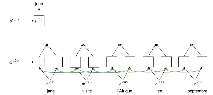
Now, the question is, If we don’t look at the whole sentence, then what part of the input French sentence should you be looking at when trying to generate this first word? For each French word, we will be looking at the words before and after it, and our Attention Model will compute set of attention weights for the nearby words, representing how much attention we should be paying for those words.

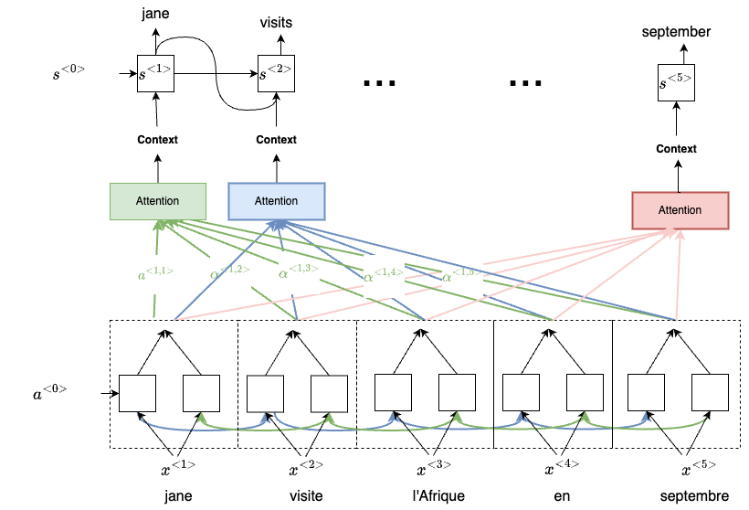
For example, we’re going to use $\alpha^{<1,1>}$ to denote the weight for the first word. This means how much attention should we be pay when generating the word. Then we’ll also come up with a second weight $\alpha^{<1,2>}$ which tells us how much attention we’re paying to this second word when translating the first word, so on and so forth.

And once we gather all weights information for the nearby words, we then feed it into the other RNN network as context for translating the first word. We then repeat the same process to generate the second, third and the rest of the words. The high-level process can be illustrated using the following diagram:

Attention model in detail

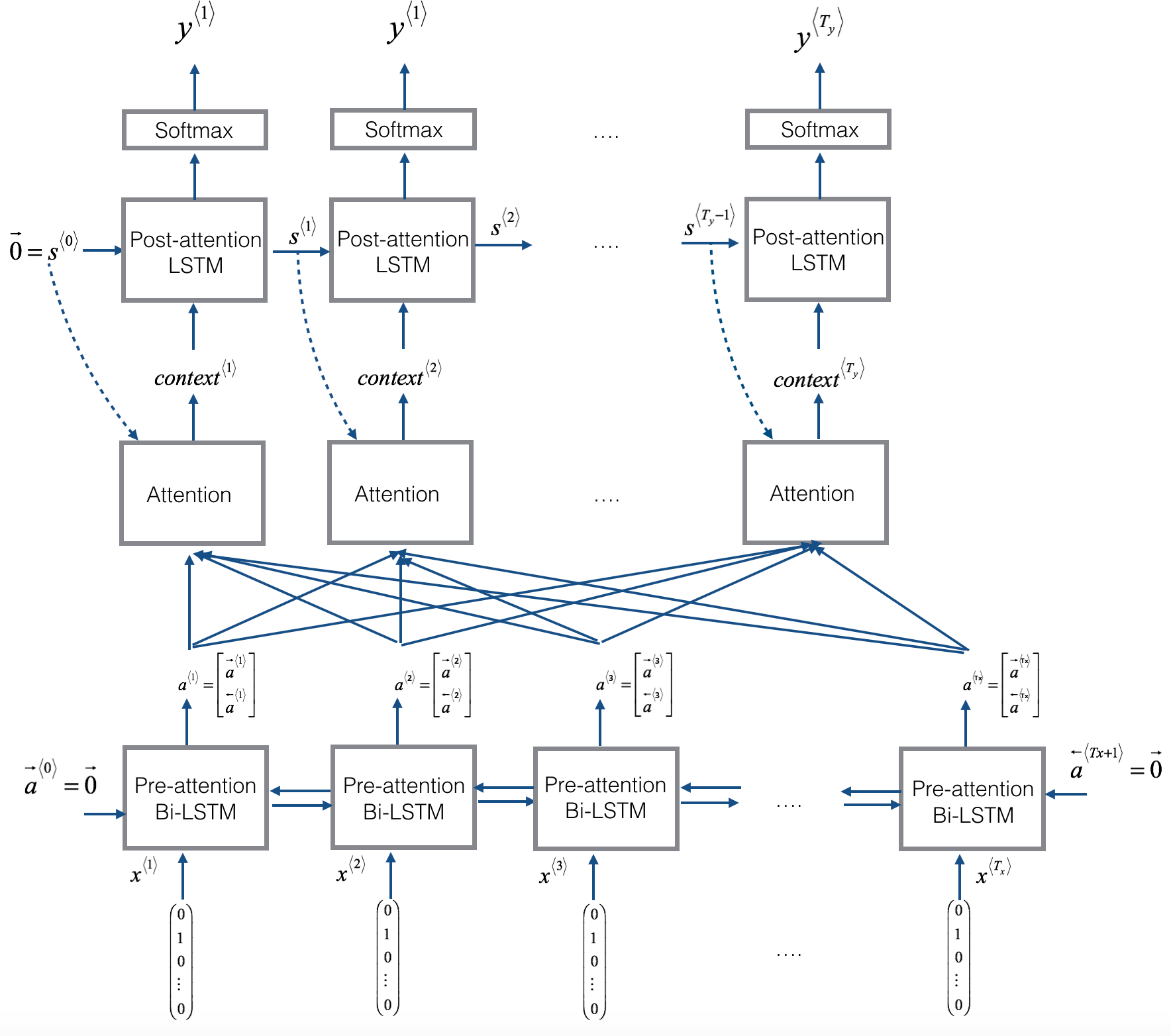
Let’s now formalize that intuition into the exact details of how you would implement an attention model. Since we have a bidirectional RNN, we use $a^{\langle t \rangle} = [\overrightarrow{a}^{\langle t \rangle}, \overleftarrow{a}^{\langle t \rangle}]$ to denote the feature vectors of each RNN block at timestamp $t$.

• $\overrightarrow{a}^{\langle t’ \rangle}$ : hidden state of the forward-direction(e.g.,pre-attention LSTM).
• $\overleftarrow{a}^{\langle t’ \rangle}$: hidden state of the backward-direction(e.g.,pre-attention LSTM).

Next, we have our forward only, a single direction RNN with state $s^{\langle t \rangle}$ to generate the translation. We use

• $y^{\langle t \rangle}$ to denote the translated word at timestamp $t$
• $context^{\langle t \rangle}$ to denote the input context at each timestamp $t$

We use the following formula to evaluate the amount of attention $y^{\langle t \rangle}$ should pay to $a^{\langle t’ \rangle}$

Next, how do we compute this $e^{\langle t,t’ \rangle}$? We could use a simple fully connected network:

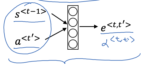
$s^{\langle t-1 \rangle}$ was the neural network state from the previous time step.

The intuition is, if you want to decide how much attention to pay to the activation of $a^{\langle t’ \rangle}$, it should depend the most on its own hidden state activation from the previous time step.

Now we should have everything to compute the context vector. The $context^{\langle t \rangle}$ is a weighted sum of the features from the different time steps weighted by these attention weights $\alpha$

Note that one downside to this approach is that it does take quadratic time or quadratic cost to run this algorithm.

To piece everything together, here is a diagram that visualize the computation process of the context vector:

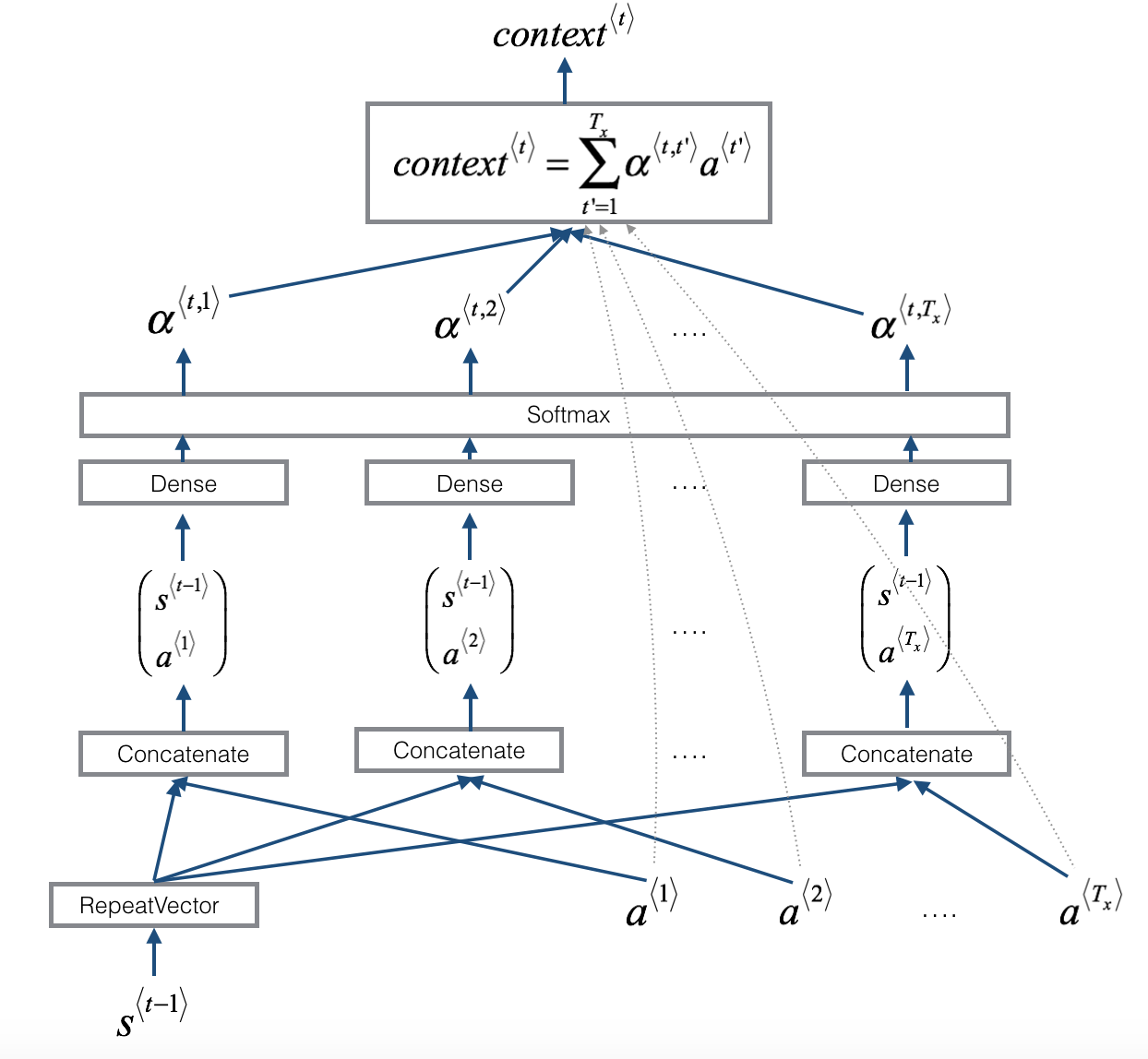
1. First, we use a RepeatVector node to copy 𝑠⟨𝑡−1⟩ 𝑇𝑥 times
2. Then we use Concatenation to concatenate 𝑠⟨𝑡−1⟩ and 𝑎⟨𝑡’⟩
3. The concatenation of 𝑠⟨𝑡−1⟩ and 𝑎⟨𝑡’⟩ is fed into a “Dense” layer, which computes 𝑒⟨𝑡, 𝑡′⟩
4. 𝑒⟨𝑡,𝑡′⟩ is then passed through a softmax to compute 𝛼⟨𝑡, 𝑡′⟩

Note that the diagram doesn’t explicitly show variable 𝑒⟨𝑡, 𝑡′⟩, but 𝑒⟨𝑡, 𝑡′⟩ is above the Dense layer and below the Softmax layer in the diagram.

Resources

• Deep Learning Specialization

Appendix #1: Attention Model Architecture