PyTorch实现GAN

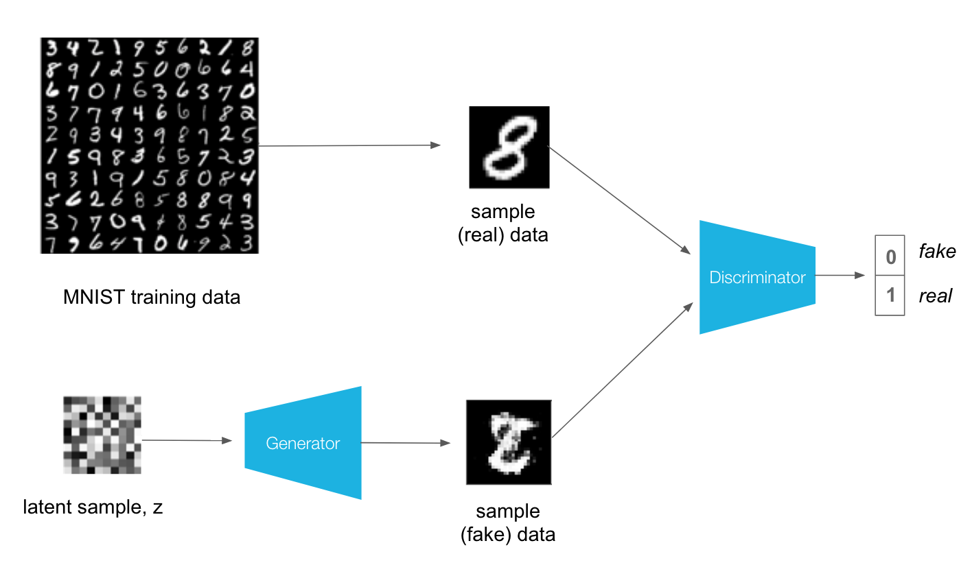
Posted on 2019-08-03 | In PyTorch , Machine Learning , Deep Learning

GAN model由两部分构成，Generator和Discriminator。 Generator的输入是一个random的tensor，它通过training不断校正自己的输出，直到输出的图片接近于真实的图片。Discriminattor是一个image classifier，用来判断输入的图片是真的还是假的。整个GAN model训练的过程可以理解为一个competition，Generator不断训练自己生成接近真实的图片，Discriminator不断训练自己检测假的图片，直到迫使Generator生成出接近真实的图片。这个过程很类似于博弈论中寻找的纳什均衡点。

The MNIST GAN Model

我们还是先从最简单的MNIST dataset开始。我们训练一个GAN model用来生成数字，整个Architecture如下所示

由于MNIST数据量比较小，我们可以使用FC layer作为hidden layer即可。对于GAN model有几个比较特殊的地方

我们需要使用Leaky ReLU作为activation函数。因为Leaky ReLU可以确保gradient可以flow through整个network。这个对于GAN model很重要，因为Generator在train的时候需要Discriminator的gradient信息。
Generator的输出通常是用tanh，将tensor限制在(-1, 1)，这是由于Generator的output通常是Discriminator的input。对于Discriminator，它输入的MNIST图片也需要映射到(-1, 1)

综上，Generator和Discriminator的model结构并不复杂，定义如下

class Discriminator(nn.Module):
    def __init__(self, input_size, hidden_dim, output_size):
        super(Discriminator, self).__init__()
        # define hidden linear layers
        self.fc1 = nn.Linear(input_size, hidden_dim*4)
        self.fc2 = nn.Linear(hidden_dim*4, hidden_dim*2)
        self.fc3 = nn.Linear(hidden_dim*2, hidden_dim)
        # final fully-connected layer
        self.fc4 = nn.Linear(hidden_dim, output_size)
        # dropout layer 
        self.dropout = nn.Dropout(0.3)

    def forward(self, x):
        # flatten image
        x = x.view(-1, 28*28)
        # all hidden layers
        x = F.leaky_relu(self.fc1(x), 0.2) # (input, negative_slope=0.2)
        x = self.dropout(x)
        x = F.leaky_relu(self.fc2(x), 0.2)
        x = self.dropout(x)
        x = F.leaky_relu(self.fc3(x), 0.2)
        x = self.dropout(x)
        # final layer
        out = self.fc4(x)
        return out

class Generator(nn.Module):

    def __init__(self, input_size, hidden_dim, output_size):
        super(Generator, self).__init__()
        # define hidden linear layers
        self.fc1 = nn.Linear(input_size, hidden_dim)
        self.fc2 = nn.Linear(hidden_dim, hidden_dim*2)
        self.fc3 = nn.Linear(hidden_dim*2, hidden_dim*4)
        # final fully-connected layer
        # restore the size to 28*28
        self.fc4 = nn.Linear(hidden_dim*4, output_size)
        # dropout layer 
        self.dropout = nn.Dropout(0.3)

    def forward(self, x):
        # all hidden layers
        x = F.leaky_relu(self.fc1(x), 0.2) # (input, negative_slope=0.2)
        x = self.dropout(x)
        x = F.leaky_relu(self.fc2(x), 0.2)
        x = self.dropout(x)
        x = F.leaky_relu(self.fc3(x), 0.2)
        x = self.dropout(x)
        # final layer with tanh applied
        out = F.tanh(self.fc4(x))
        return out

Discriminator和Generator的HyperParameter定义如下

Discriminator(
  (fc1): Linear(in_features=784, out_features=128, bias=True)
  (fc2): Linear(in_features=128, out_features=64, bias=True)
  (fc3): Linear(in_features=64, out_features=32, bias=True)
  (fc4): Linear(in_features=32, out_features=1, bias=True)
  (dropout): Dropout(p=0.3, inplace=False)
)

Generator(
  (fc1): Linear(in_features=100, out_features=32, bias=True)
  (fc2): Linear(in_features=32, out_features=64, bias=True)
  (fc3): Linear(in_features=64, out_features=128, bias=True)
  (fc4): Linear(in_features=128, out_features=784, bias=True)
  (dropout): Dropout(p=0.3, inplace=False)
)

Train Discriminator

在Training时，我们要同时计算来自Generator和Discriminator的两个loss。其中Discriminator比较直观，因为它的输出是0或者1，代表出图片是真还是假，因此它是一个binary classifier。其loss函数可以用binary cross-entropy loss。这里有一个比较tricky的地方，我们需要用BCEWithLogitsLoss而不是sigmoid + BCELoss

prob = F.sigmoid(logits) #logits是最后一个FC的输出
loss != nn.BCELoss(prob, labels)
loss =  nn.BCEWithLogitsLoss(prob, labels*0.9)

BCEWithLogitsLoss combines a sigmoid activation function and and binary cross entropy loss in one function.

对于Discriminator来说，它有两个inputs，一个是real image，一个是fake image。因此它也有两个loss函数，real_loss和fake_loss。对于real image，groud truth label是1，即D(real_image)=1，这里为了让model更generalize，我们另y=0.9。对于输入是fake image，我们希望D(fake_image)=0，因此y是0。总的loss为real_loss + fake_loss。定义loss函数如下

def real_loss(D_out, smooth=False):
    batch_size = D_out.size(0)
    # label smoothing
    if smooth:
        # smooth, real labels = 0.9
        labels = torch.ones(batch_size)*0.9
    else:
        labels = torch.ones(batch_size) # real labels = 1
        
    # numerically stable loss
    criterion = nn.BCEWithLogitsLoss()
    # calculate loss
    loss = criterion(D_out.squeeze(), labels)
    return loss

def fake_loss(D_out):
    batch_size = D_out.size(0)
    labels = torch.zeros(batch_size) # fake labels = 0
    criterion = nn.BCEWithLogitsLoss()
    # calculate loss
    loss = criterion(D_out.squeeze(), labels)
    return loss

训练Discriminator，可以follow下面步骤

d_optimizer.zero_grad()
# 1. Compute the discriminator loss on real, training images
D_real = D(real_images)
d_real_loss = real_loss(D_real, smooth=True)
# 2. Generate fake images
z = np.random.uniform(-1, 1, size=(batch_size, z_size))
z = torch.from_numpy(z).float()
fake_images = G(z)
# 3. Compute the discriminator losses on fake images        
D_fake = D(fake_images)
d_fake_loss = fake_loss(D_fake)
#4.  add up loss and perform backprop
d_loss = d_real_loss + d_fake_loss
#5. back prop + optimization
d_loss.backward()
d_optimizer.step()

Train Generator

对于Generator来说，它的输出y是一个fake image，我们将它作为Discriminator的输入。由于Generator的目标是D(fake_image)=1，我们需要让Discriminator认为来自Generator的输入是一个real image，因此我们需要用real_loss

训练Generator，可以follow下面的步骤

g_optimizer.zero_grad()        
# 1. Generate fake images
z = np.random.uniform(-1, 1, size=(batch_size, z_size))
z = torch.from_numpy(z).float()
fake_images = G(z)

# 2. Compute the discriminator losses on fake images 
# using flipped labels!
D_fake = D(fake_images)
g_loss = real_loss(D_fake) # use real loss to flip labels

# 3. perform backprop
g_loss.backward()
g_optimizer.step()

Training Results

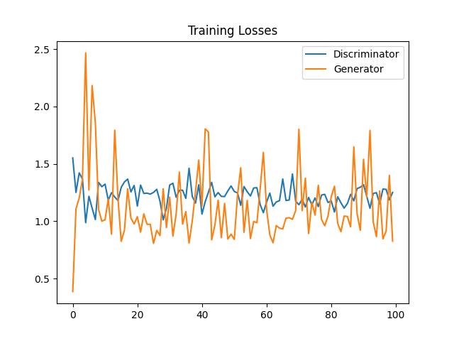
我们选取optimizer为Adam, learning rate为0.002, num_epochs = 100 两个model的training loss的变化如下图

我们也可以观察在训练中Generator输出的变化情况。我们可以在每个epoch之后输出一张Generator的图片

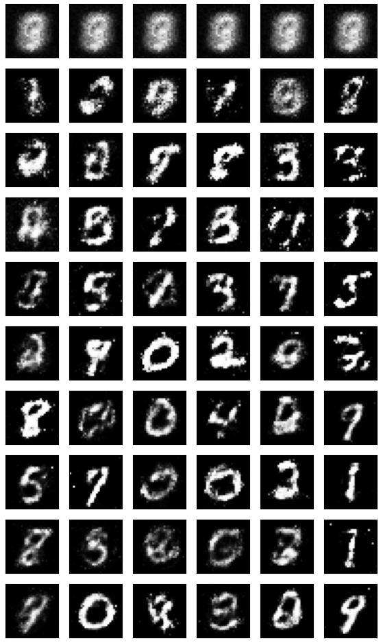
可见，对于任意一个random tensor，Generator可以生成一个类似手写的数字。当然MNIST是个非常简单的情况，对于复杂一点的图片，我们需要用Convolution layer来代替FC layer。

Deep Convolutional GAN

DC GAN和上面的MNIST model工作原理基本相同，不同的是DC GAN使用conv layer作为hidden layer。Paper中还列出了architecture设计的几个关键点

Replace any pooling layers with strided convolutions (discriminator) and fractional-strided convolutions (generator).
Use batchnorm in both the generator and the discriminator.
Remove fully connected hidden layers for deeper architectures.
Use ReLU activation in generator for all layers except for the output, which uses Tanh.
Use LeakyReLU activation in the discriminator for all layers.

Discriminator

Discriminator的结构和上面的MNIST model类似，它由若干个conv layer构成。和普通的classification model不同的是，它用stride=2的conv来取代pooling。

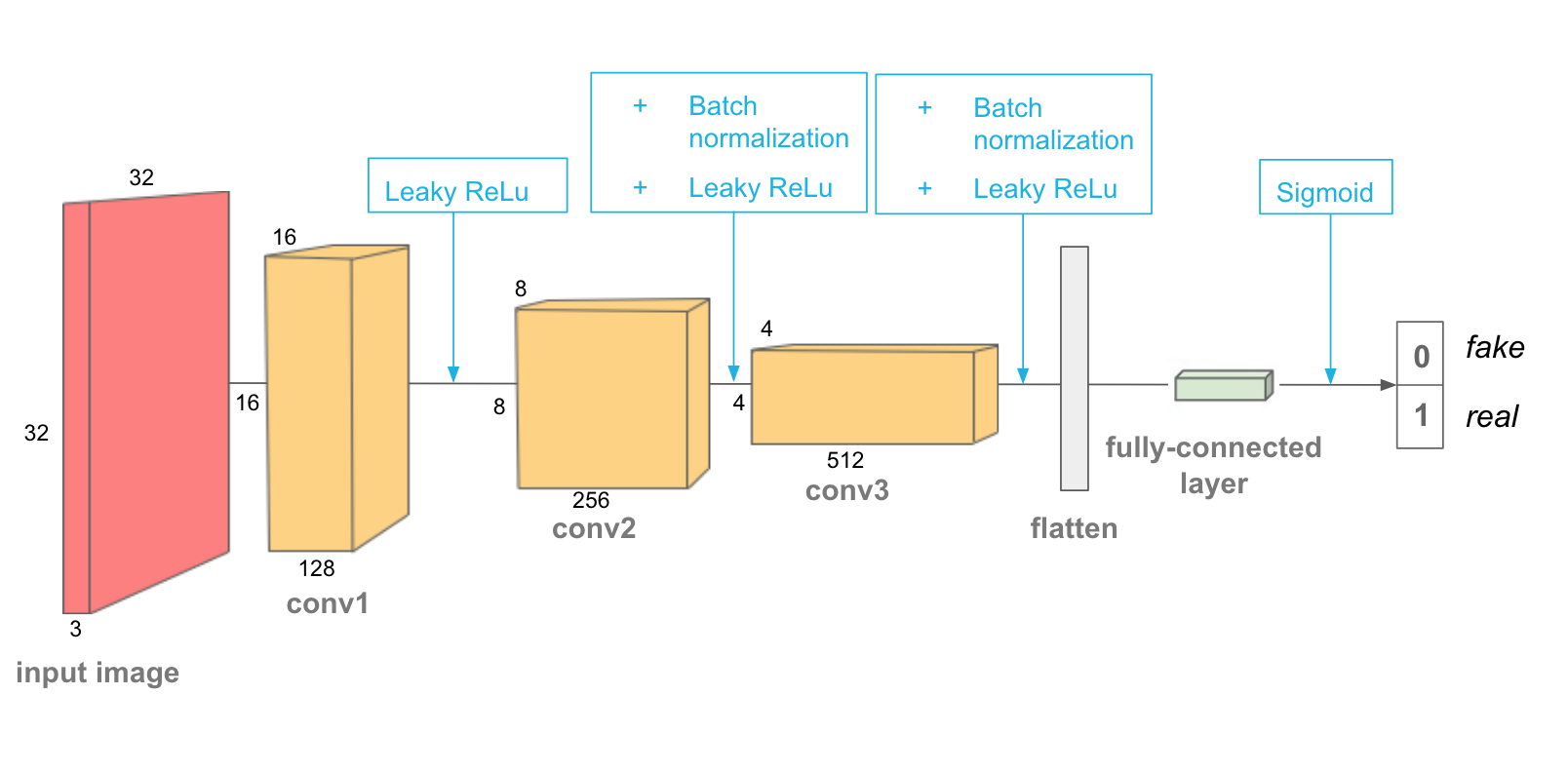
需要注意的是，除了第一个conv layer外，后面的每个conv layer都需要追加BatchNorm操作来帮助training更好的converge。conv layer的depth可以从32开始，后面逐层double (64, 128, etc)。

# helper conv function
def conv(in_channels, out_channels, kernel_size, stride=2, padding=1, batch_norm=True):
    """Creates a convolutional layer, with optional batch normalization.
    """
    layers = []
    conv_layer = nn.Conv2d(in_channels, out_channels, 
                           kernel_size, stride, padding, bias=False)
    # append conv layer
    layers.append(conv_layer)
    if batch_norm:
        # append batchnorm layer
        layers.append(nn.BatchNorm2d(out_channels))
    # using Sequential container
    return nn.Sequential(*layers)

class Discriminator(nn.Module):
    def __init__(self, conv_dim=32):
        super(Discriminator, self).__init__()
        self.conv_dim = conv_dim
        self.conv1 = conv(3, conv_dim, 4, batch_norm=False)
        self.conv2 = conv(conv_dim, conv_dim*2, 4)                
        self.conv3 = conv(conv_dim*2, conv_dim*4, 4)
        self.fc = (conv_dim*4*4*4, 1)
        
    def forward(self, x):
        # complete forward function
        x = F.leaky_relu(self.conv1(x), 0.2)
        x = F.leaky_relu(self.conv2(x), 0.2)
        x = F.leaky_relu(self.conv3(x), 0.2)
        x = x.view(-1, self.conv_dim*4 * 4 * 4)
        x = self.fc(x)
        return x

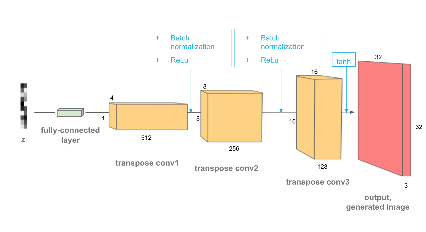
Generator

Generator的input也是一个noise vector，它使用transpose conv(stride=2)来增加feature map的spatial size。同样的，我们需要使用对conv layer追加BatchNorm

# helper deconv function
def deconv(in_channels, out_channels, kernel_size, stride=2, padding=1, batch_norm=True):
    """Creates a transposed-convolutional layer, with optional batch normalization.
    """
    layers = []
    transposed_conv_layer = nn.ConvTranspose2d(in_channels, out_channels, 
                           kernel_size, stride, padding, bias=False)
    # append conv layer
    layers.append(transposed_conv_layer)
    if batch_norm:
        # append batchnorm layer
        layers.append(nn.BatchNorm2d(out_channels))
    # using Sequential container
    return nn.Sequential(*layers)
        

class Generator(nn.Module):
    def __init__(self, z_size, conv_dim=32):
        super(Generator, self).__init__()
        self.conv_dim = conv_dim
        # complete init function
        self.fc = nn.Linear(z_size, conv_dim*4*4*4)
        self.deconv1 = deconv(conv_dim*4, conv_dim*2, 4)
        self.deconv2 = deconv(conv_dim*2, conv_dim, 4)
        self.deconv3 = deconv(conv_dim, 3, 4, batch_norm = False)
        
    def forward(self, x):
        x = self.fc(x)
        x = x.view(-1, self.conv_dim*4, 4, 4) # (1, 128, 4, 4)
        x = F.relu(self.deconv1(x), 0.2) # (1, 64, 8, 8)
        x = F.relu(self.deconv2(x), 0.2) # (1, 32, 16, 16)
        x = self.deconv3(x) #(32, 32)
        x = F.tanh(x)
        
        return x

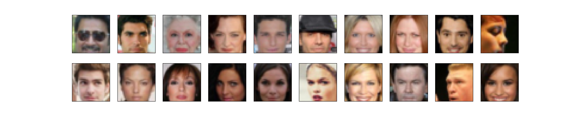
Generate Faces

我们可以用上面的model来尝试生成人脸，CelebFaces提供了大量的图片，为了节省训练时间，我们将图片resize成(32,32)，Sample如下图所示

生成图片如下图所示

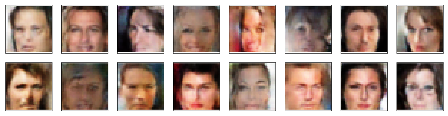
不论是MNIST GAN还是DC GAN，他们model的结构都不复杂，而且他们的输入都是一个noise vector。实际应用中，这种model并没有特别大用处，想要生成高质量的fake image，仅仅使用random input是不够的，接下来我们来看一下Cycle GAN。

Cycle GAN

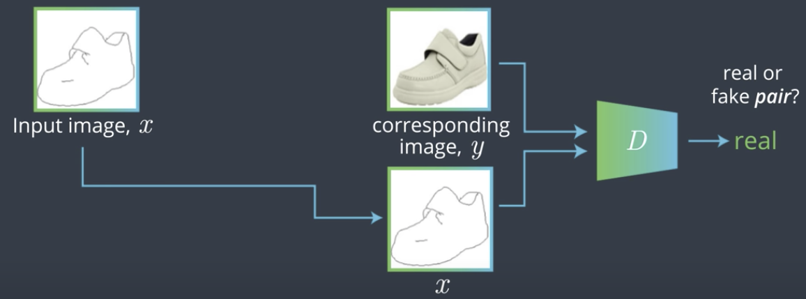
在了解Cycle GAN之前，我们先要了解下Pix2Pix GAN。Pix2Pix GAN解决的问题是image mapping，即Generator将一张图片x映射成另一张图片y。这就需要我们的training data是pair images。其中，$x_i$是Generator的输入，$y_i$是ground true。我们的目标是训练Generator，使$G(x_i) = y_i$。

Paper使用Unet作为Generator的architecture。Input先经过一个encoder变成小的feature maps，再经过decoder将尺寸复原。

decoder输出的图片再通过Discriminator进行classification。Discriminator的结构和前一篇文章中的DC GAN类似

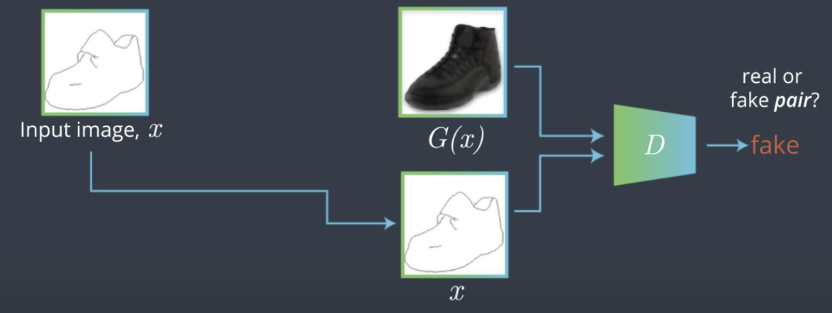
上面Generator结构有一个问题是，Discriminator如何判断Generator的输出是否是fake。举例来说，理想情况下，$G(x_1)=y_1$，但是如果出现$G(x_1)=y_2$的情况，由于$y_2$是real image，Discriminator也会将其判定为true。因此，Discriminator的输入应该是一对pair，它的outputs是这对pair是否是match。如下图所示

实际应用中，这种一对一的pair data是很难得到的。比较容易得到的是两组image set - $X$和$Y$，比如一组马的图片和一组斑马的图片。此时我们需要找到一个映射使 $G(X) = Y$，即对于$X$中的每个image，都有$G(x) = y$。此时不是一对一的映射，而是多对多的映射，是unsupervised learning，如下图所示

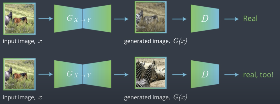
如果仔细思考，这里会有一个问题，既然是多对多，就会有多个$x$映射到同一个$y$的可能，为了避免这种情况，我们还要建立一个反向约束，即$G(Y) = X$，此时有

$G_{YtoX}(G_{XtoY(x)}) \approx x$

既然需要reverse mapping，我们就需要两组GAN，一组完成$G(X)=Y$，另一组完成$G(Y)=X$。因此我们就有两组Adversarial Loss $L_X$和$L_Y$。此外，为了满足上面的式子，我们还需要引入一个Cycle Consistency Loss来确保生成出的图片被revert回去后可以和原图近似。

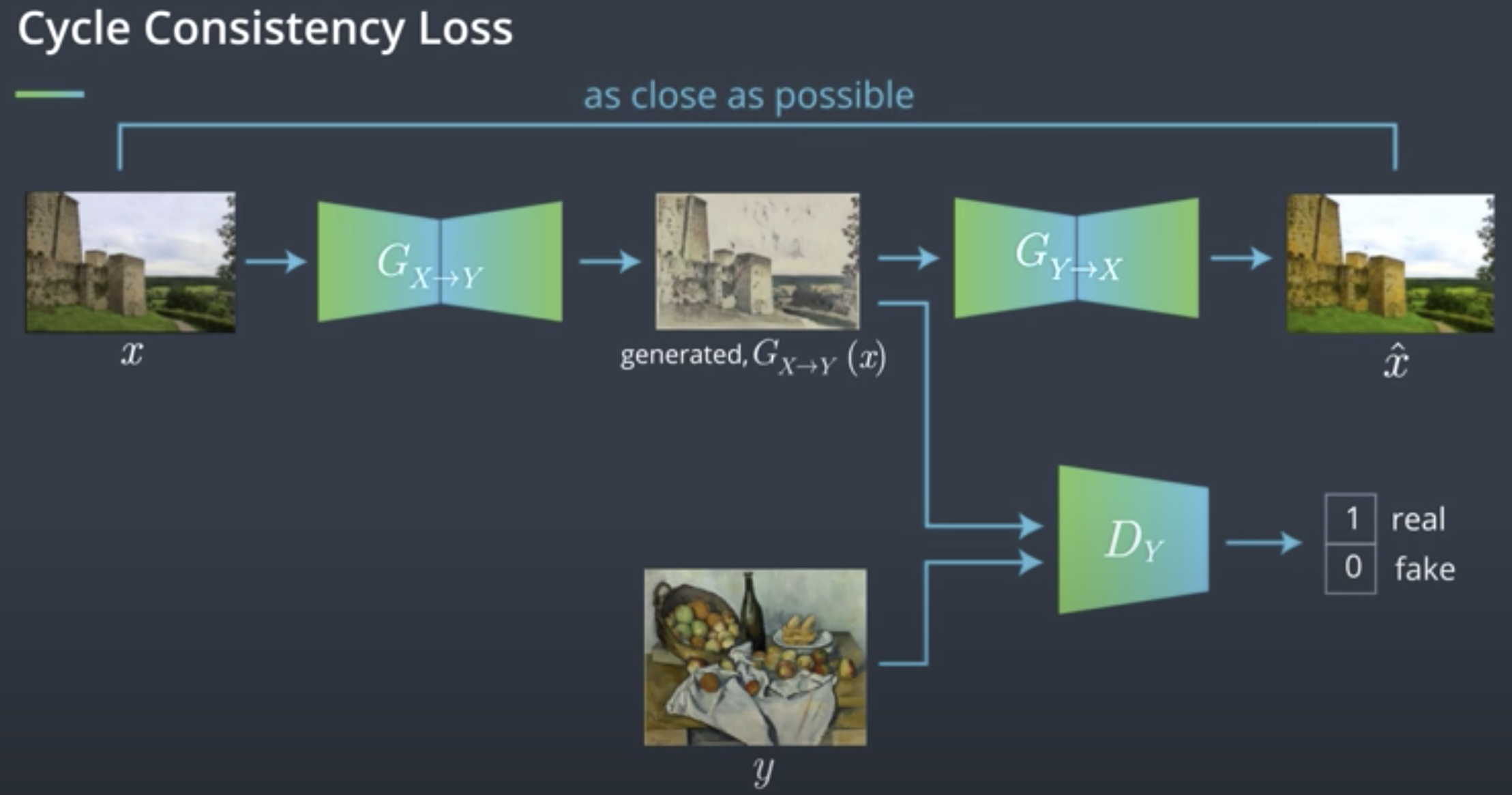
Cycle Consistency Loss同样也有两组，分别为forward consistency loss 和 backward consistency loss，分别对应$x$和$y$。

$total loss = L_Y + L_X + \lambda L_{cyc}$

Discriminator

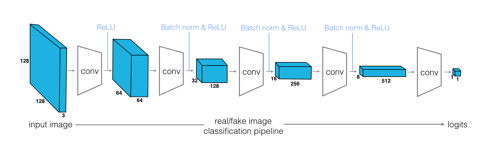
Cycle GAN需要两个Discriminator和Generator。Discriminator的结构前文DC GAN相似，区别在于Input不需要经过Fully Connected Layer。我们另input的size为[1, 3, 128, 128]

class Discriminator(nn.Module):
    def __init__(self, conv_dim=64):
        super(Discriminator, self).__init__()
        # Should accept an RGB image as input and output a single value
        self.conv_dim = conv_dim
        self.conv1 = conv(3, conv_dim, 4, batch_norm=False) #(64, 64, 64)
        self.conv2 = conv(conv_dim, conv_dim * 2, 4) # (32, 32, 128)
        self.conv3 = conv(conv_dim * 2, conv_dim * 4, 4) # (16, 16, 256)
        self.conv4 = conv(conv_dim * 4, conv_dim * 8, 4) # (8, 8, 512)
        self.conv5 = conv(conv_dim * 8, 1, 4, stride=1, batch_norm=False)

    def forward(self, x):
        # define feedforward behavior
        x = F.relu(self.conv1(x))
        x = F.relu(self.conv2(x))
        x = F.relu(self.conv3(x))
        x = F.relu(self.conv4(x))
        x = self.conv5(x)
        return x

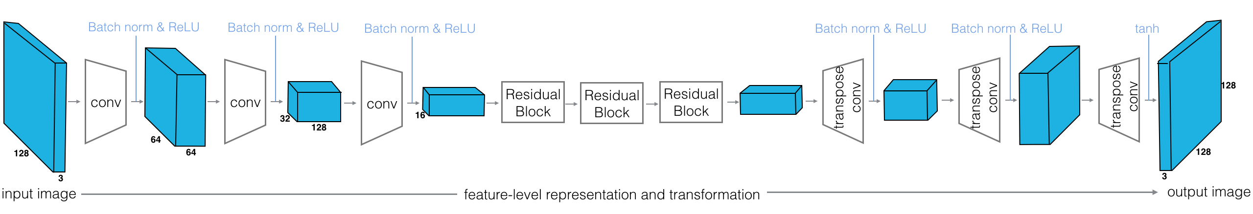
Generator

Generator的结构有一点特殊，我们需要在encoder和decoder之间引入skip connection，即Residual Block。其目的是解决梯度消失的问题，一个Residual block定义如下

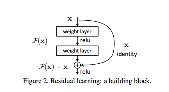
通常一个block有两个conv组成，每个conv使用3x3的kernel，且input和output的channel相同，因此当x通过两个conv的layer之后，得到的y的shape不会发生任何变化，因此可以和x进行elementwise相加。

class ResidualBlock(nn.Module):
    """Defines a residual block.
       This adds an input x to a convolutional layer (applied to x) with the same size input and output.
       These blocks allow a model to learn an effective transformation from one domain to another.
    """
    def __init__(self, conv_dim):
        super(ResidualBlock, self).__init__()
        self.conv1 = conv(conv_dim, conv_dim, kernel_size=3, stride=1, padding=1, batch_norm=True)
        self.conv2 = conv(conv_dim, conv_dim, kernel_size=3, stride=1, padding=1, batch_norm=True)
        
    def forward(self, x):
        y = F.relu(self.conv1(x))
        y = x + self.conv2(y)
        return y

接下来我们根据前面提到的Generator的结构创建model，paper中使用6个residual block，input size同样为[1,3,128,128]

class CycleGenerator(nn.Module):
    def __init__(self, conv_dim=64, n_res_blocks=6):
        super(CycleGenerator, self).__init__()
        # 1. Define the encoder part of the generator
        self.conv1 = conv(3, conv_dim, 4)
        self.conv2 = conv(conv_dim, conv_dim*2, 4)
        self.conv3 = conv(conv_dim*2, conv_dim*4, 4)
        # 2. Define the resnet part of the generator
        res = []
        for _ in range(n_res_blocks):
            res.append(ResidualBlock(conv_dim * 4))
        self.res_blocks = nn.Sequential(*res)
        # 3. Define the decoder part of the generator
        self.deconv1 = deconv(conv_dim*4, conv_dim*2, 4)
        self.deconv2 = deconv(conv_dim*2, conv_dim, 4)
        self.deconv3 = deconv(conv_dim, 3, 4, batch_norm=False)

    def forward(self, x):
        x = F.relu(self.conv1(x))
        x = F.relu(self.conv2(x))
        x = F.relu(self.conv3(x))
        x = self.res_blocks(x)
        x = F.relu(self.deconv1(x))
        x = F.relu(self.deconv2(x))
        x = F.tanh(self.deconv3(x))
        return x

Discriminator and Generator Losses

前面提到，Cycle GAN的loss由两部分组成，一部分是Adversarial loss，前面文章已经讨论过，但是Cycle GAN的Discriminator不能使用Cross Entropy loss，原因paper中提到会有梯度消失的问题，因此，这里需要使用mean square loss. Cycle GAN loss的另一分部分是Cycle Consistency loss，这个loss比较简单，只是比较生成的图片和原图片每个像素点的差异即可。各种loss计算如下

def real_mse_loss(D_out):
    # how close is the produced output from being "real"?
    return torch.mean((D_out-1)**2)

def fake_mse_loss(D_out):
    # how close is the produced output from being "false"?
    return torch.mean(D_out**2)

def cycle_consistency_loss(real_im, reconstructed_im, lambda_weight):
    # calculate reconstruction loss 
    # as absolute value difference between the real and reconstructed images
    reconstr_loss = torch.mean(torch.abs(real_im - reconstructed_im))
    # return weighted loss
    return lambda_weight*reconstr_loss   

训练Discriminator

训练Discriminator的步骤和前文的DC GAN基本类似，不同的是Cycle GAN要train两个Discriminator用来判断X和Y。可以follow下面步骤

##   First: D_X, real and fake loss components   ##
# Train with real images
d_x_optimizer.zero_grad()
# 1. Compute the discriminator losses on real images
out_x = D_X(images_X)
D_X_real_loss = real_mse_loss(out_x)
# Train with fake images
# 2. Generate fake images that look like domain X based on real images in domain Y
fake_X = G_YtoX(images_Y)
# 3. Compute the fake loss for D_X
out_x = D_X(fake_X)
D_X_fake_loss = fake_mse_loss(out_x)
# 4. Compute the total loss and perform backprop
d_x_loss = D_X_real_loss + D_X_fake_loss
d_x_loss.backward()
d_x_optimizer.step()

##   Second: D_Y, real and fake loss components   ##
# Train with real images
d_y_optimizer.zero_grad()
# 1. Compute the discriminator losses on real images
out_y = D_Y(images_Y)
D_Y_real_loss = real_mse_loss(out_y)
# Train with fake images
# 2. Generate fake images that look like domain Y based on real images in domain X
fake_Y = G_XtoY(images_X)
# 3. Compute the fake loss for D_Y
out_y = D_Y(fake_Y)
D_Y_fake_loss = fake_mse_loss(out_y)
# 4. Compute the total loss and perform backprop
d_y_loss = D_Y_real_loss + D_Y_fake_loss
d_y_loss.backward()
d_y_optimizer.step()

PyTorch实现GAN

The MNIST GAN Model

Train Discriminator

Train Generator

Training Results

Deep Convolutional GAN

Discriminator

Generator

Generate Faces

Cycle GAN

Discriminator

Generator

Discriminator and Generator Losses

训练Discriminator

Resources