The Self-Attention Mechanism

The Self-Attention Intuition

Let’s say we have the following french sentence:

Jane visite l'Afrique en septembre

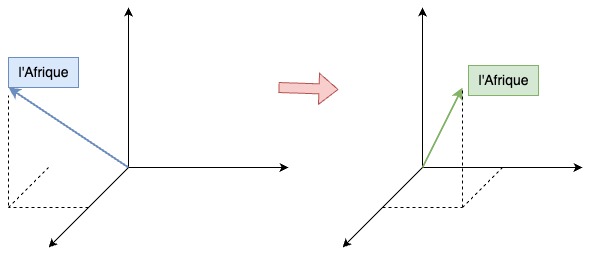
Our goal will be computing an attention-based representation for each word $A^{\langle i \rangle}$. For example, one way to represent l'Afrique would be to just look up the word embedding for l'Afrique. But depending on the context, are we thinking of l'Afrique or Africa as a site of historical interests or as a holiday destination, or as the world’s second-largest continent. Depending on how you're thinking of `l'Afrique`, you may choose to represent it differently, and that's what this representation $A^{\langle 3 \rangle}$ will do .

Self-Attention will look at the surrounding words to try to figure out what does "l'Afrique" really mean in this sentence, and find the most appropriate representation for this.

Semantically, This means changing the position of l'Afrique’s embedding vector in the high dimensional space, moving the vector to the place where it can best represent its meaning in the sentence.

Formal Definition

Mathematically, We use the following formula to calculate the attention representation for each word:

In the formula, A(q, K, V) is the attention-based vector representation of a word. We have $q^{\langle i \rangle}$, $k^{\langle i \rangle}$ and $v^{\langle i \rangle}$, representing query, key and value. $\sqrt{d_k}$ is added for numerical stability, doesn’t carry specific meanings.

Computation Process Visualization

To best understand what the formula means, let’s take a look at another sentence:

a fluffy blue creature roamed the verdant forest

Initially, every word has its own initial embedding that only encodes the meaning of that particular word (let’s ignore the positional encoding for now). Let’s denote the initial embedding vector as $\vec{E}_i$, our goal is to find $\vec{E}_i’$ that captures the real meaning of each word in the sentence.

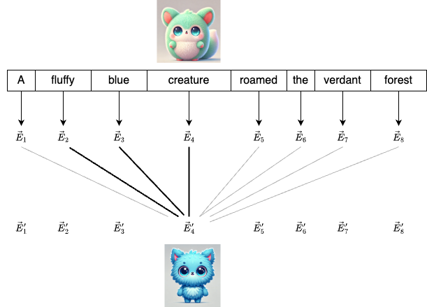
Take the word “creature” as an example. The adjectives “fluffy” and “blue” contribute more to the meaning of “creature” than other surrounding words. As a result, “creature” should pay more attention to these words.

The Attention Pattern

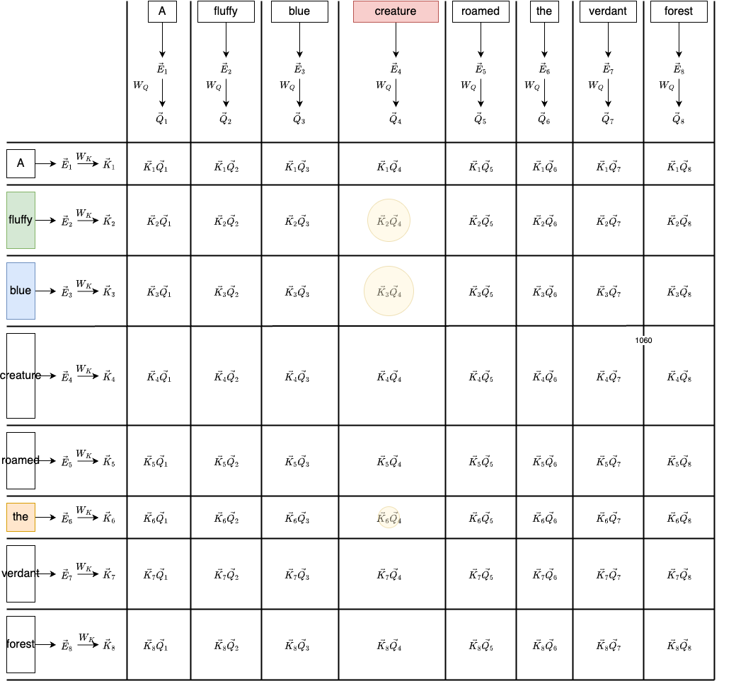
In the high-dimensional embedding space, this means that the query vector for “creature” is more similar to the key vectors of “fluffy” and “blue”. We can think of a key vector as an answer to a query vector. When a key and a query matches, they will align closely in the embedding space. To measure how well each key matches each query, we compute the dot product between the query vectors and the key vectors:

Recall that the dot product between two vectors is proportional to their cosine similarity - assuming the vectors are normalized

This is what the matrix multiplication $Q K^\top$ represents: each entry is the dot product between a query and a key, indicating how much one word should attend to another. In our case, the dot products between “creature” and “fluffy” or “blue” should be greater than other words(e.g. “the”).

To create query vector for the words, we need a matrix $W_Q$ to multiply their corresponding embedding vector:

Note that, the $W_Q$ has a much smaller dimension than the embedding vector. If the embedding vector size is [8, 122888] (8 words, each word is 122888 dimension), then the $W_Q$ could be [12288, 128], so the $\vec{Q_i}$ is a [8, 128] vector.

Similarly, to create a key vector for the words, we need a matrix $W_K$ multiply the embedding vector:

The $W_K$ has the same dimension as $W_Q$ ([12288, 128]). The $\vec{Q_i}$ is also a [8, 128] vector. Thus, when multiplying $QK^T$, we will get a [8, 8] matrix as shown above.

Note that The results of the dot products between the query and key vectors range from $-\infty$ to $\infty$ However, what we want is a probability distribution that tells us how much attention should be paid to each key vector. To achieve this, we apply the softmax function, which turns the raw scores into positive values and scales them, so they add up to 1, forming a valid probability distribution.

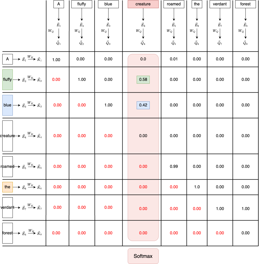
At this point, we have explained the meaning of $\text{softmax}\left(\frac{Q K^\top}{\sqrt{d_k}}\right)$, in the next section, we will explore the value matrix and see it updates the embedding vectors.

Masking

Another important note is that the Self-Attention can look at words before and after the word of interest. However, in a decoder-only model(GPT), you never want to allow later words to influence earlier words, since otherwise they could give away the answer for what comes next.

The Masked Self-Attention ignores anything that comes after the word of interest. This means in our attention pattern table, the ones representing later tokens influencing earlier ones need to be zero.

To calculate mask self-attention, we just need to add the mask matrix to the scaled similarities:

At a high level, the way this works is that we apply masking before the softmax function by replacing certain dot product values (the words that comes after the current word) with $-\infty$.

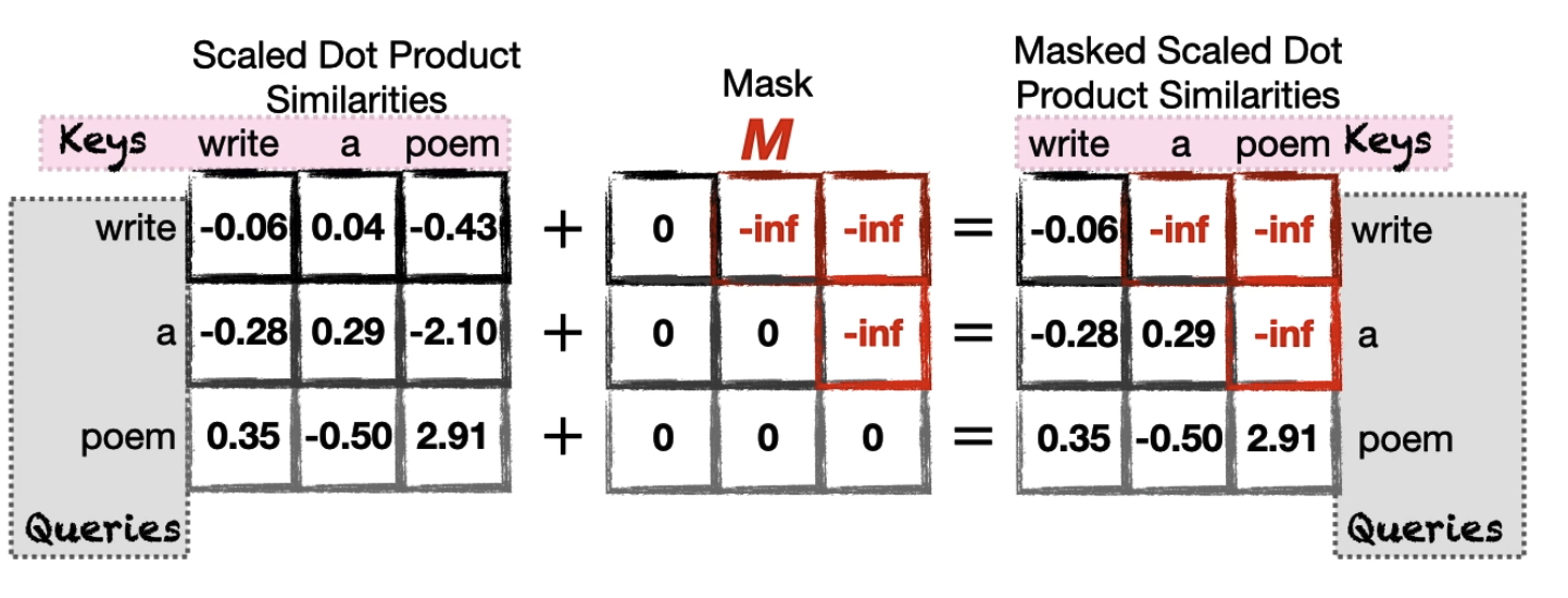
After applying softmax, these values effectively become zero, meaning they contribute nothing to the final attention distribution — while still preserving a valid probability distribution over the remaining (unmasked) positions.

Updating the embedding vectors

Great, the attention pattern lets the model deduce which words are relevant to which other words. Now we need to update the actual embeddings. For example, we want the embedding of “fluffy” to somehow cause a change to “creature” that moves it to a different position in the high dimensional space.

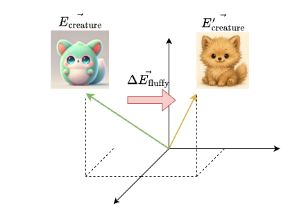
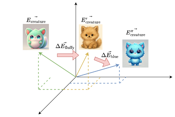
To achieve this, we will be using a third matrix $W_v$, which is called the value matrix. This matrix is multiplied by the embedding of that first word(“fluffy”), producing a value vector $\vec{\Delta E}$. This vector represents the contribution from “fluffy”, and we add it to the embedding of “creature”:

This moves “creature”’s embedding vector to a desired position in the high dimensional space. We then repeat the same process for the word “blue”, and eventually, these contributions shift the position of “creature” to its best location in the high dimensional embedding space.

To generalize this process, let’s go back to the attention pattern diagram:

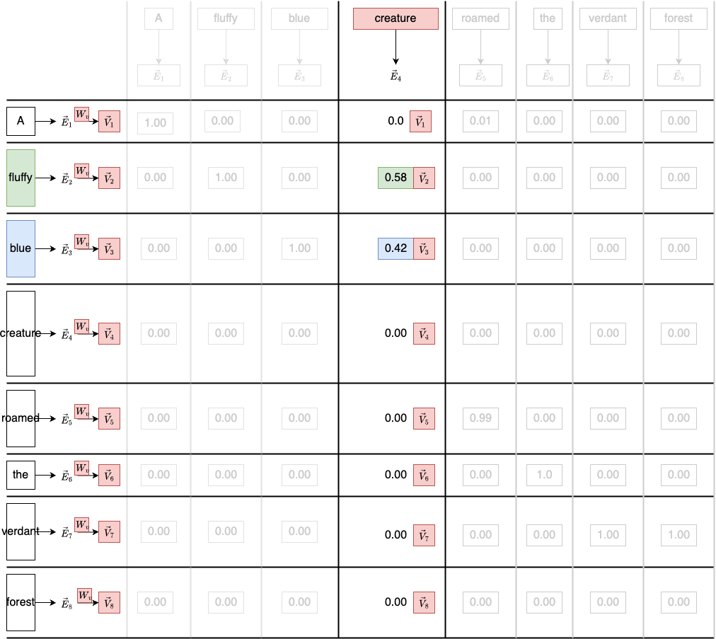
For each row in the diagram, we multiply the embedding each of the embedding vector by the value matrix $W_v$. Let’s say the embedding vector size is [8, 12288], then the size of $W_v$ is [12288, 12288]. This gives us a [8, 12288] value vector.

Note that the number column for $W_V$ determines the number of dimensions in the final attention representation of the word. In practice, this number is usually the same as the embedding dimension. We can think of it as repositioning the original word in embedding space so that it reflects what’s important in context.

For each column in the diagram, we multiply each value vectors by the corresponding weight in that column. Recall that the weight is just the softmax result of the dot product. The weighted sum produces a $\vec{\Delta E_{\text{creature}}}$

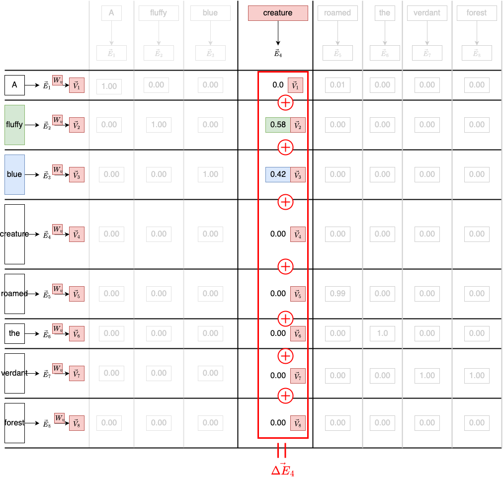
This gives us the self-attention score for the word “creature”. Finally, we can update the embedding vector for “creature” with this score - $\vec{\Delta E_{\text{creature}}}$

This has completed the process for computing the attention representation of the word “creature”. Now, we just need to apply the same weighted sum across all the columns for all the words, producing a sequence of $\vec{\Delta E_i}$. And we add all those value vectors to the corresponding embeddings, producing a full sequence of more refined embeddings.

Zooming out, this whole process is described as a single head of self-attention. This process is parameterized by three distinct matrices, all filled with tunable parameters, the key, the query, and the value:

Before wrapping up the single self-attention unit, there is one more thing that can help us understand how it works as a black box. Let’s look at the PyTorch code below:

# define the emebdding dimension
EmbeddingDims = 256

encodings_matrix = torch.randn(8, EmbeddingDims)
print("Encoding Matrix:", encodings_matrix.shape) # torch.Size([8, 256])

selfAttention = SelfAttention(d_model=EmbeddingDims)
# forward pass
attention_values = selfAttention.forward(encodings_matrix)
print("Attention values:", attention_scores.shape) # torch.Size([8, 256])

If we treat the attention unit as a module(SelfAttention), the input is a (N, D1) tensor, and the output is a (N, D2). In most of the cases, we have D1 == D2, this means, we just transform the original embedding vector to a new embedding vector in the same dimension space.

Multi-Head Attention

In the above discussion, we have explained the single head self-attention in great detail. However, in order to correctly establish how words are related in longer more complicated sentences and paragraphs, we can apply the single self-attention block multiple times simultaneously.

GPT3 for example uses 96 attention heads inside each block

Each attention unit is called a head and has its own sets of weights for calculating the queries, keys and values. In the example below, we have two embedding vectors as inputs, and we have three self-attention heads:

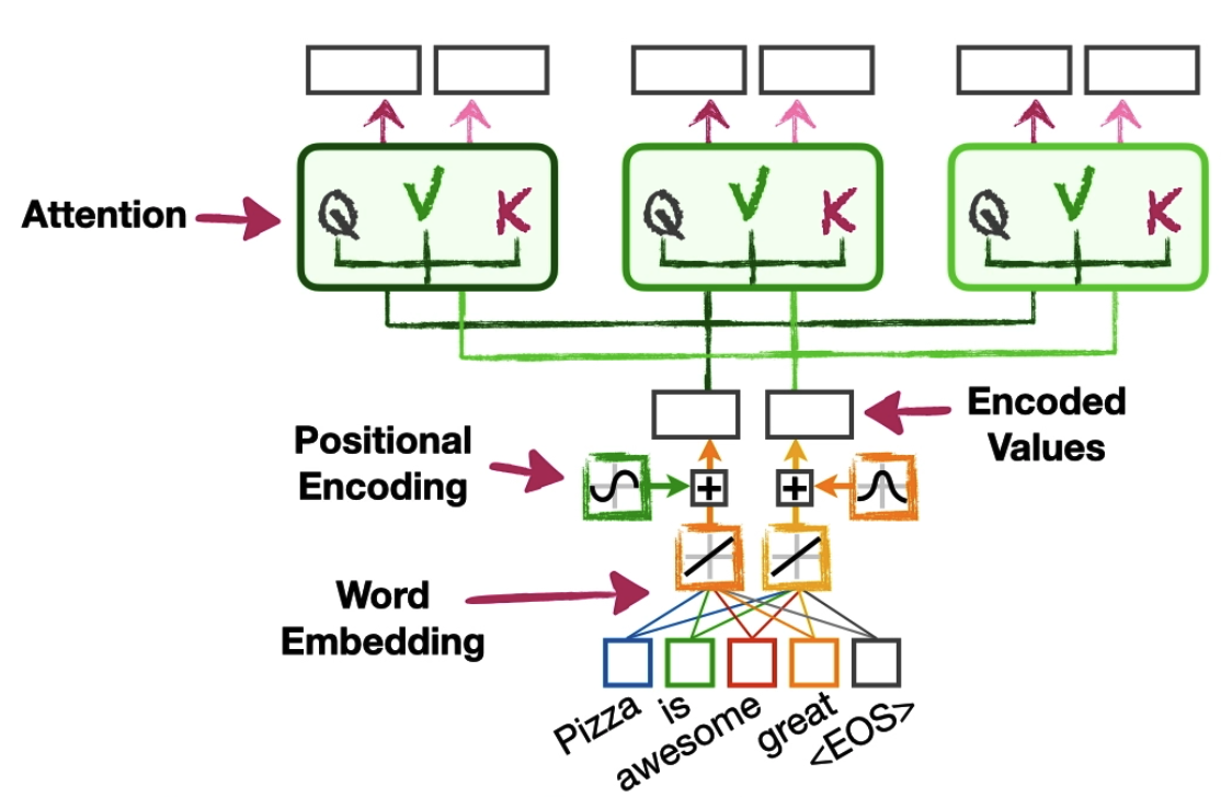
We can imagine that each attention head will nudge the words embedding to desired positions in a high dimensional space. The multi-head attention is simply repeating this process multiple times, nudging the words embeddings from different contextual perspectives in parallel.

Grouped Query Attention Head

More recently, grouped query attention is proposed to allow us to share the same Keys and Values by a group of attention heads (Query is not shared). This can help reduce the number of parameters that the model needs to train while preserve the accuracy of the prediction.

In Meta’s recent paper - The Llama 3 Herd of Models, they outline their model architecture as follows:

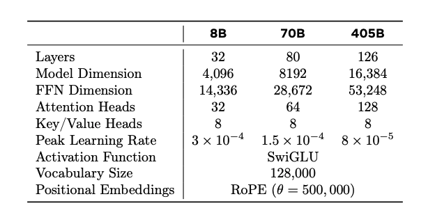
Note that the number of attention heads is 32 and the number of key/value heads is 8. The paper also mentions that they use grouped query attention with 8 key-value heads to improve inference speed and to reduce the size of key-value caches during decoding. So this means, the n_groups = 8 and the n_attention_heads = 32, resulting in 4 attention heads per group.

We will talk more about other parameters in this paper in the second part of the transformer block in the next post.

Summary

In summary, the self-attention head does two things:

1. Relevant scoring: Assigning a score to how relevant each of the input are to the token we’re currently processing.

2. Combining information: combine the scores to produce an attention representation(a new embedding vector) for each word in the sentence.

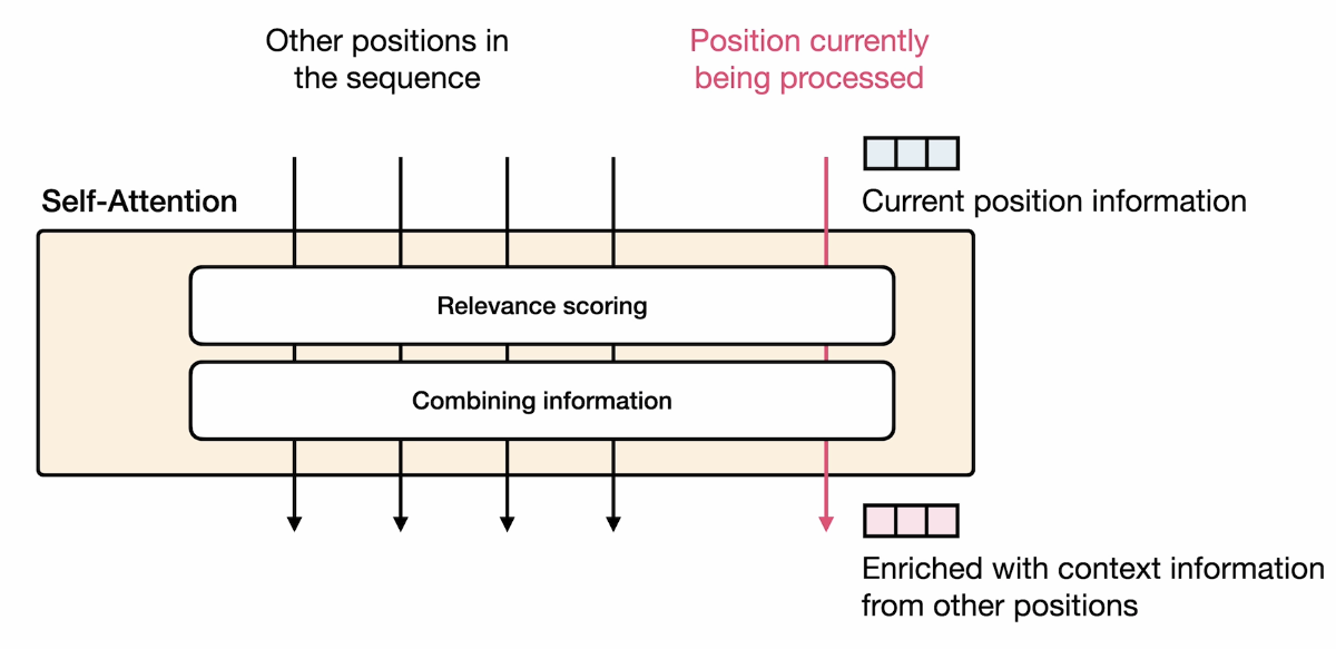
Now we have the attention representation for each word in our sentence, how do we use with them to predict the next word? In the next post, we will discuss the second part of the transformer block, and we will see how the embeddings get used in the downstream of the network.

Resources

• Deep Learning Specialization
• How Transformer LLMs work
• Attention in Transformers: Concept and Code in PyTorch
• 3 blues 1 brown: Attention in Transformers

Appendix #1: PyTorch implementation of a single self-attention head

import torch
import torch.nn as nn
import torch.nn.functional as F

EmbeddingDims = 256

class SelfAttention(nn.Module): 
                            
    def __init__(self, 
                d_model=EmbeddingDims,  
                 row_dim=0, 
                 col_dim=1):
        ## d_model = the number of embedding values per token.
        ##           Because we want to be able to do the math by hand, we've
        ##           the default value for d_model=2.
        ##           However, in "Attention Is All You Need" d_model=512
        ##
        ## row_dim, col_dim = the indices we should use to access rows or columns
        super().__init__()
        
        ## Initialize the Weights (W) that we'll use to create the
        ## query (q), key (k) and value (v) for each token
        self.W_q = nn.Linear(in_features=EmbeddingDims, out_features=128, bias=False)
        self.W_k = nn.Linear(in_features=EmbeddingDims, out_features=128, bias=False)
        self.W_v = nn.Linear(in_features=EmbeddingDims, out_features=EmbeddingDims, bias=False)
        
        self.row_dim = row_dim
        self.col_dim = col_dim

        
    def forward(self, token_encodings):
        ## token_encodings: word_embedding + positional encoding
        ## Create the query, key and values using the encoding numbers
        ## associated with each token (token encodings)
        q = self.W_q(token_encodings)
        k = self.W_k(token_encodings)
        v = self.W_v(token_encodings)

        ## Compute similarities scores: (q * k^T)
        ## transpose swap the two dimensions: dim0, dim1 = dim1, dim0
        sims = torch.matmul(q, k.transpose(dim0=self.row_dim, dim1=self.col_dim))
        print(sims.shape)

        ## Scale the similarities by dividing by sqrt(k.col_dim)
        scaled_sims = sims / torch.tensor(k.size(self.col_dim)**0.5)

        ## Apply softmax to determine what percent of each tokens' value to
        ## use in the final attention values.
        attention_percents = F.softmax(scaled_sims, dim=self.col_dim)
        print(attention_percents.shape)

        ## Scale the values by their associated percentages and add them up.
        attention_scores = torch.matmul(attention_percents, v)

        return attention_scores

def main():
    # 8 words, 256 embedding values per word
    encodings_matrix = torch.randn(8, EmbeddingDims)
    print("Encoding Matrix:", encodings_matrix.shape)

    selfAttention = SelfAttention(d_model=EmbeddingDims)
    attention_values = selfAttention(encodings_matrix)
    print("Attention values:", attention_scores.shape)


if __name__ == "__main__":
    main()

Appendix #2: PyTorch implementation of a multi-head self-attention

class MultiHeadAttention(nn.Module):
    def __init__(self, 
                 d_model=2,  
                 row_dim=0, 
                 col_dim=1, 
                 num_heads=1):
        
        super().__init__()

        ## create a bunch of attention heads
        self.heads = nn.ModuleList(
            [SelfAttention(d_model, row_dim, col_dim) 
             for _ in range(num_heads)]
        )

        self.col_dim = col_dim
        
    def forward(self, 
                encodings_for_q, 
                encodings_for_k,
                encodings_for_v):

        ## run the data through all of the attention heads
        return torch.cat([head(encodings_for_q, 
                               encodings_for_k,
                               encodings_for_v) 
                          for head in self.heads], dim=self.col_dim)