LLM Fine-tuning and evaluation

Posted on 2024-11-24 | In GenAI , Transformer , LLM

Limitations of in-context learning

May not work for smaller models
Examples take up space in the context window

LLM fine-tuning at a high level

In contrast to pre-training, where you train the LLM using vast amounts of unstructured textual data via self-supervised learning, fine-tuning is a supervised learning process where you use a data set of labeled examples to update the weights of the LLM. The labeled examples are prompt completion pairs, the fine-tuning process extends the training of the model to improve its ability to generate good completions for a specific task.

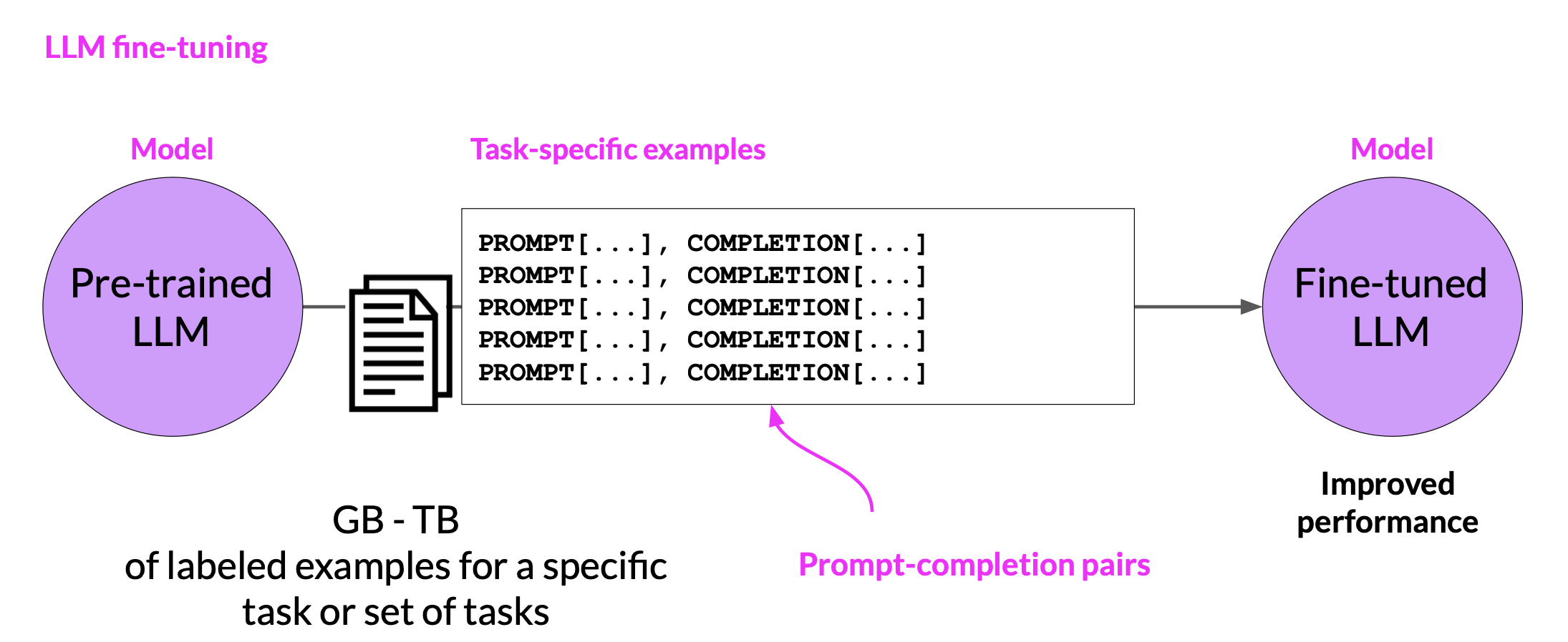
One strategy, known as instruction fine-tuning, is particularly good at improving a model’s performance on a variety of tasks.

Fine Tuning using prompts

Instruction fine-tuning trains the model using examples that demonstrate how it should respond to a specific instruction

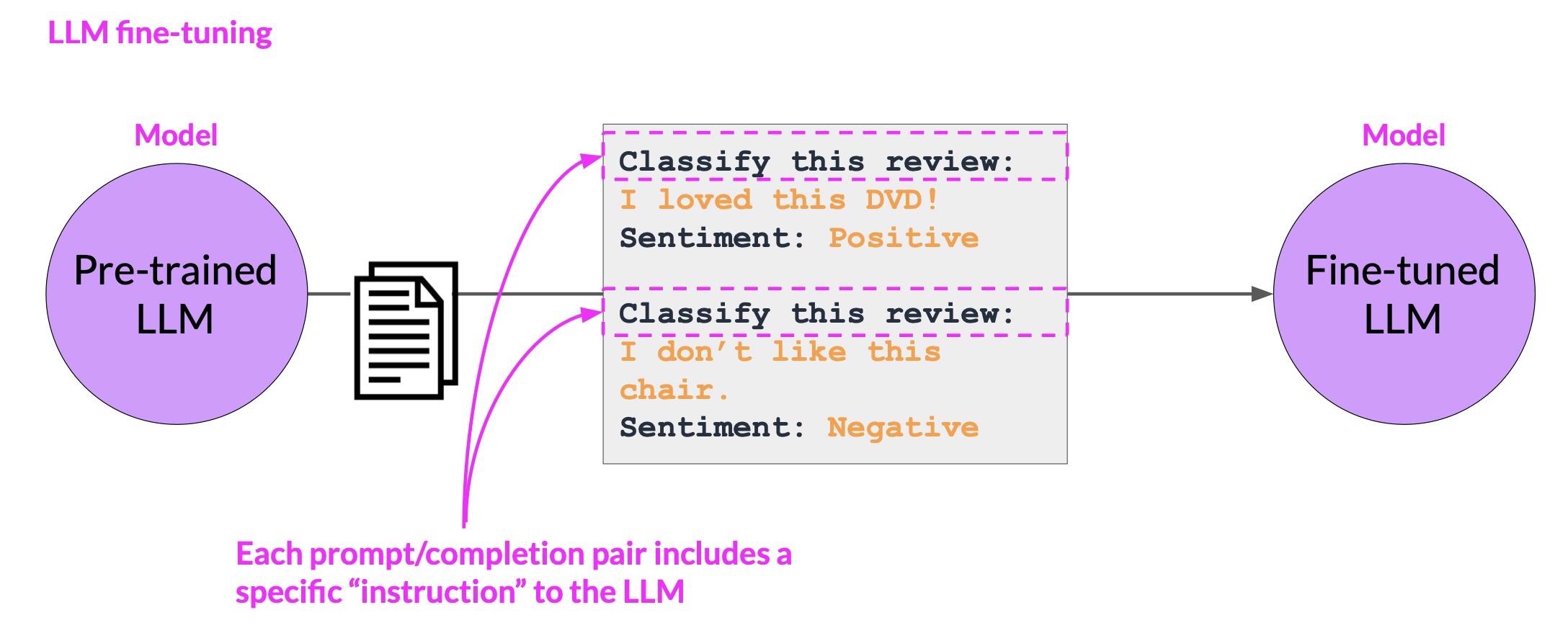
For example, if you want to fine tune your model to improve its summarization ability, you’d build up a data set of examples that begin with the instruction summarize, the following text or a similar phrase. And if you are improving the model’s translation skills, your examples would include instructions like translate this sentence.

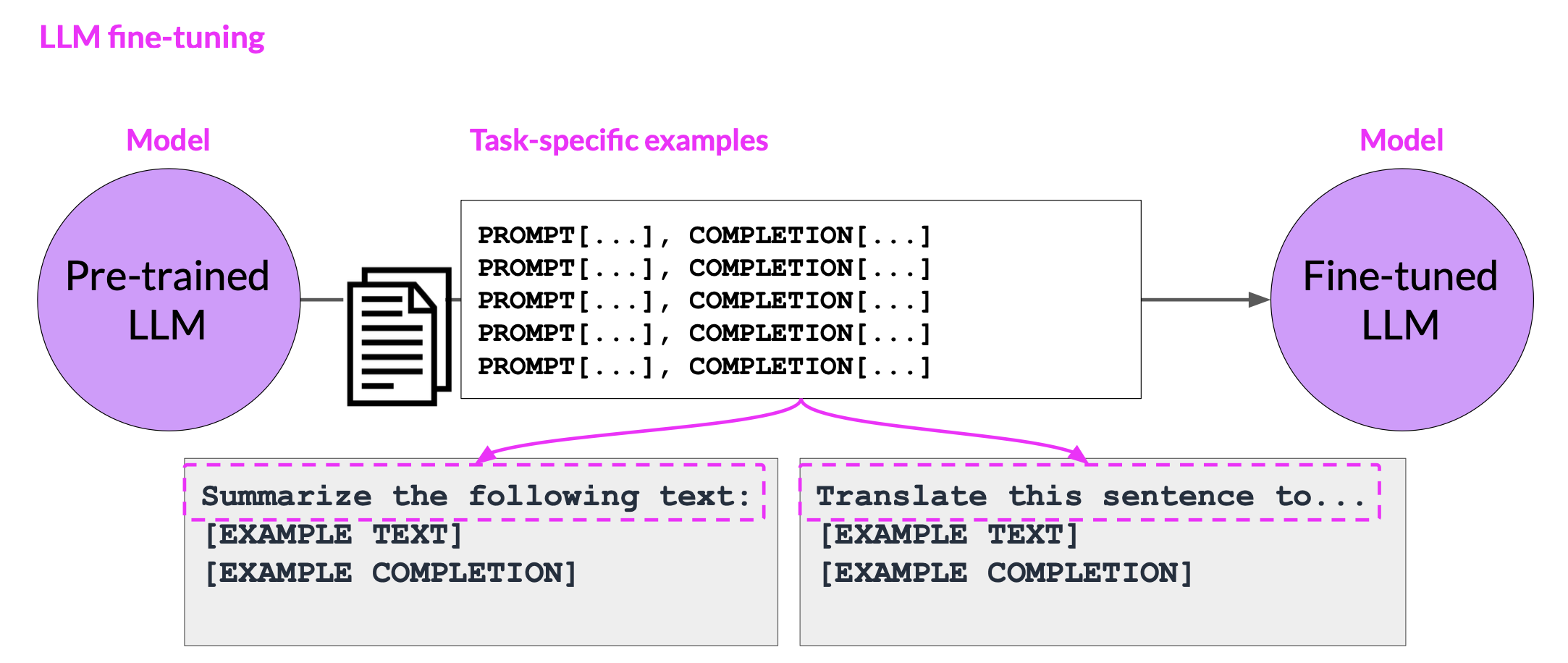
These prompt completion examples allow the model to learn to generate responses that follow the given instructions.

Instruction fine-tuning, where all of the model’s weights are updated is known as full fine-tuning. The process results in a new version of the model with updated weights

The fine-tuning process

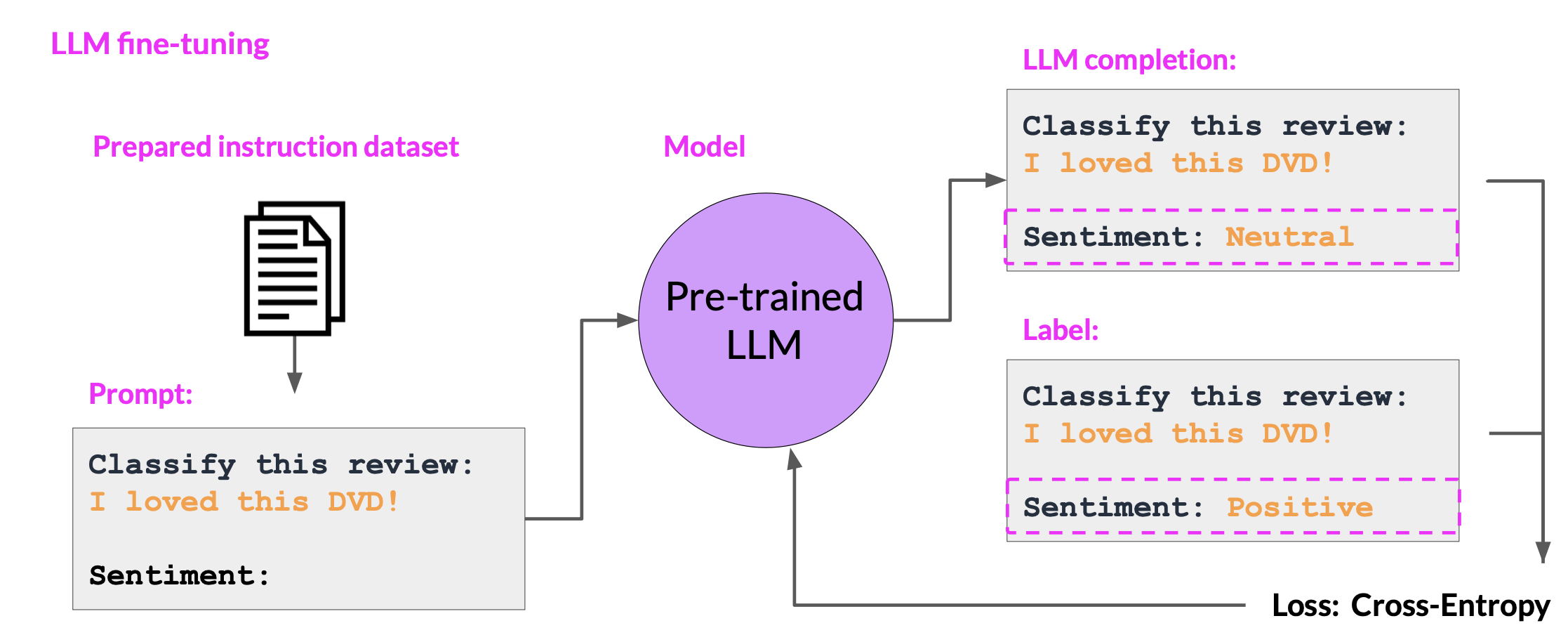
During fine-tuning, you select prompts from your training data set and pass them to the LLM, which then generates completions.
Next, you compare the LLM completion with the response specified in the training data. You can see here that the model didn’t do a great job, it classified the review as neutral, which is a bit of an understatement. The review is clearly very positive. Remember that the output of an LLM is a probability distribution across tokens. So you can compare the distribution of the completion and that of the training label and use the standard cross entropy function to calculate loss between the two token distributions.
Then use the calculated loss to update your model weights in standard back propagation. You’ll do this for many batches of prompt completion pairs and over several epochs, update the weights so that the model’s performance on the task improves
After you’ve completed your fine tuning, you can perform a final performance evaluation using the holdout test data set. This will give you the test accuracy.

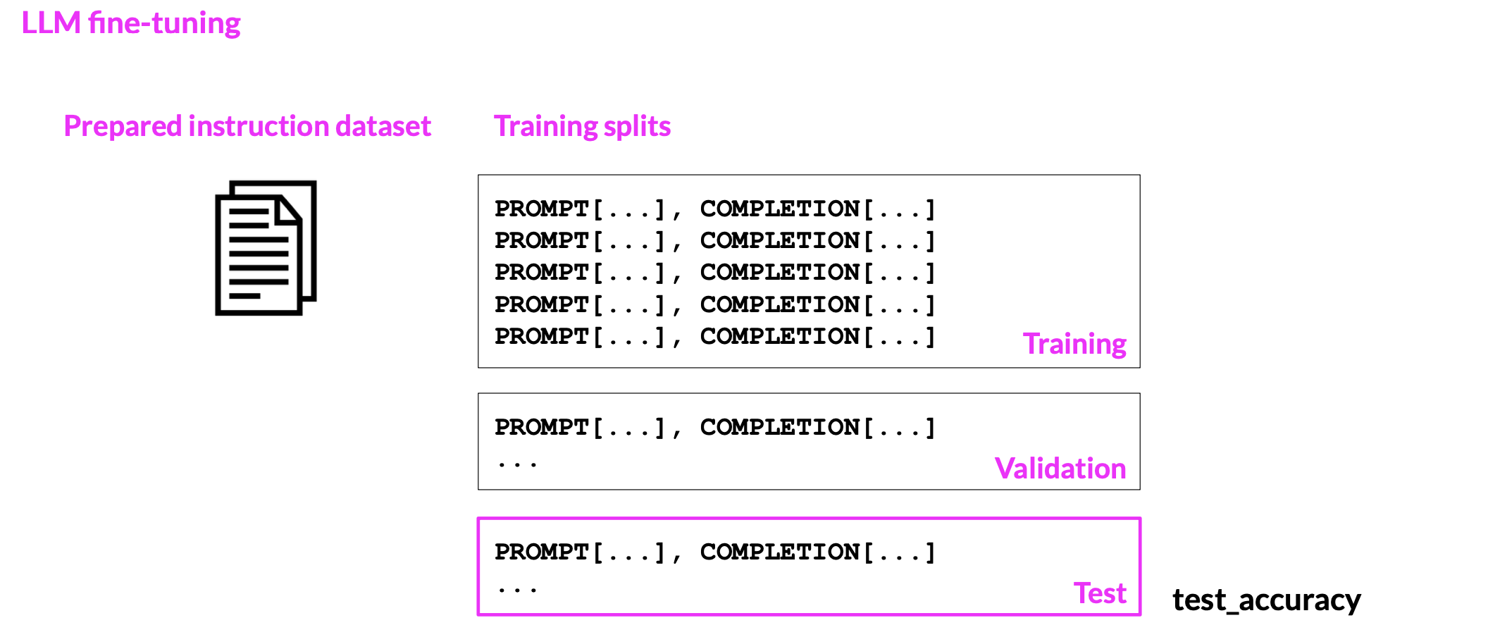
Fine-tuning with instruction prompts is the most common way to fine-tune LLMs these days. From this point on, when you hear or see the term fine-tuning, you can assume that it always means instruction fine tuning.

Catastrophic forgetting

While the fine-tuning process allows the model to have a better performance on a single task, it can degrade performance on other tasks. This is called catastrophic forgetting.

Catastrophic forgetting happens because the full fine-tuning process modifies the weights of the original LLM.

For example, while fine-tuning can improve the ability of a model to perform sentiment analysis on a review and result in a quality completion, the model may forget how to carry out named entity recognition.

How to avoid catastrophic forgetting

First note that you might not have to!
Fine-tune on multiple tasks at the same time
Consider Parameter Efficient Fine-tuning(PEFT)
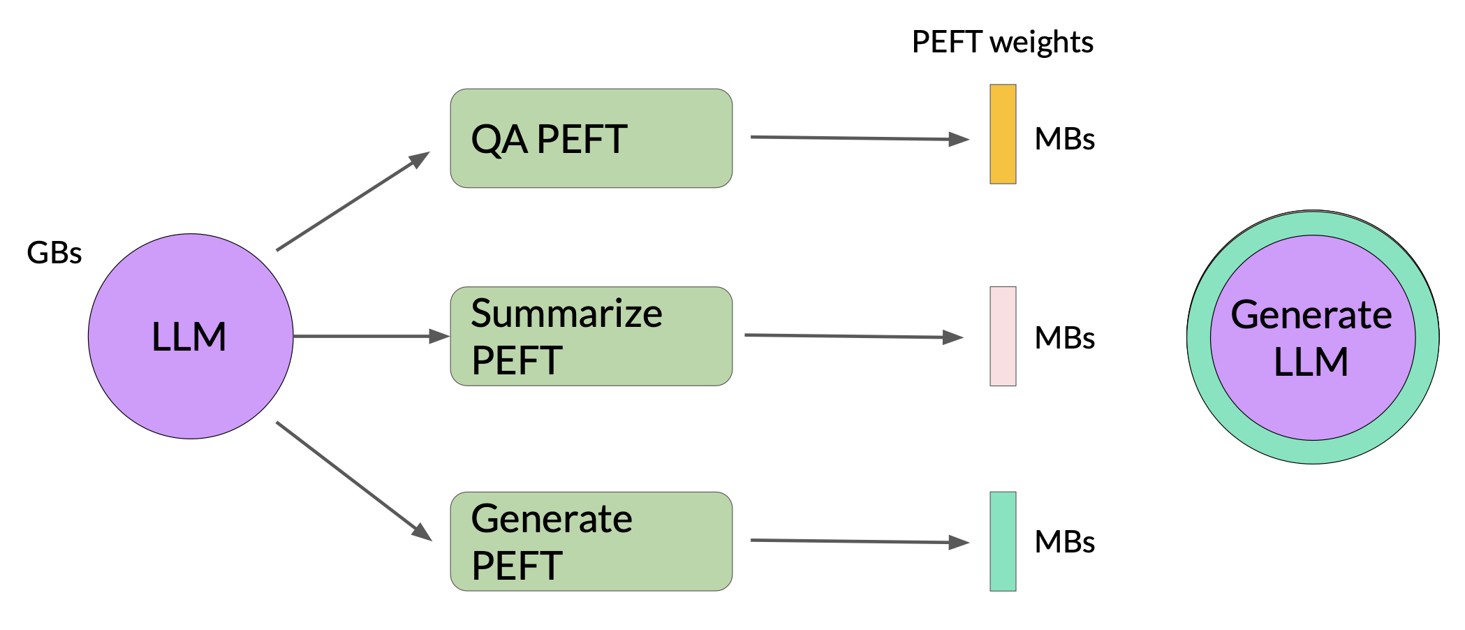
- PEFT is a set of techniques that preserves the weights of the original LLM and trains only a small number of task-specific adapter layers and parameters.

Multi-task, instruction fine-tuning

Multitask fine-tuning is an extension of single task fine-tuning, where the training dataset is a composed of example inputs and outputs for multiple tasks.

Here, the dataset contains examples that instruct the model to carry out a variety of tasks, including summarization, review rating, code translation, and entity recognition. You train the model on this mixed dataset so that it can improve the performance of the model on all the tasks simultaneously, thus avoiding the issue of catastrophic forgetting

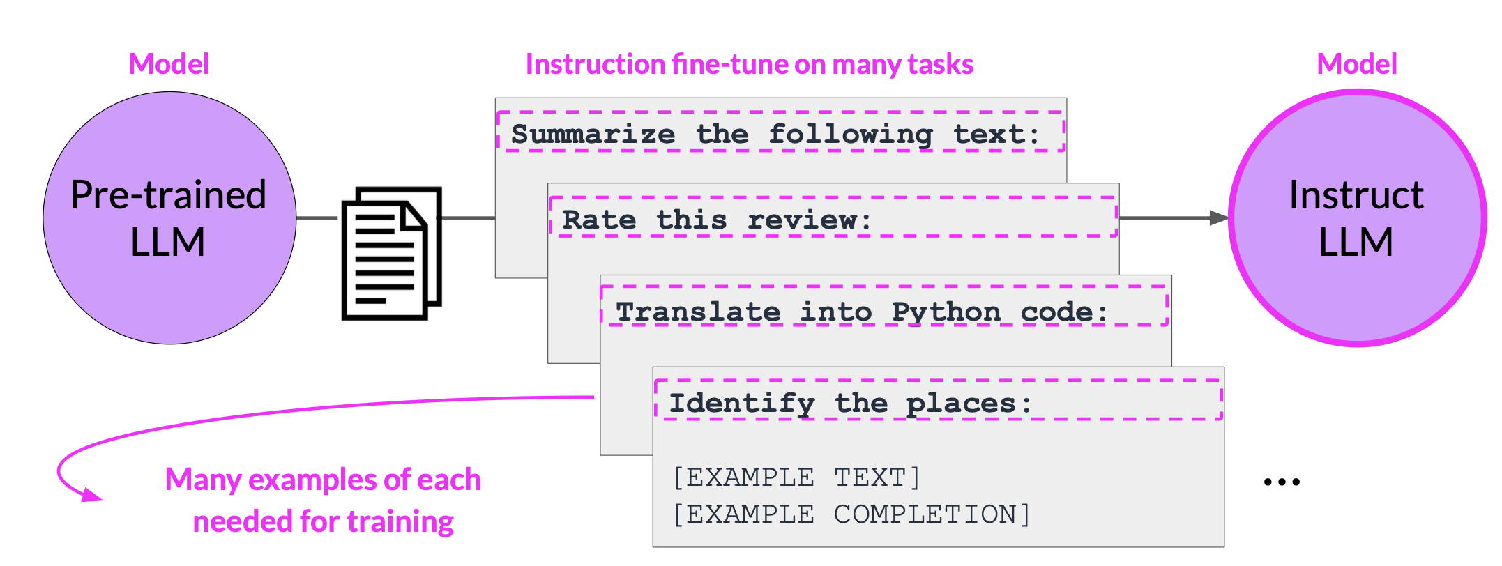
One drawback to multitask fine-tuning is that it requires a lot of data. You may need as many as 50-100,000 examples in your training set.

Model Evaluation metrics

In traditional machine learning, you can assess how well a model is doing by looking at its prediction accuracy because the models are deterministic.

\[\text{Accuracy} = \frac{\text{Correct Predictions}}{\text{Total Predictions}}\]

But with large language models where the output is non-deterministic and language-based evaluation is much more challenging. We need an automated, structured way to make measurements. ROUGE and BLEU, are two widely used evaluation metrics for different tasks.

ROUGE(Recall Oriented Under Study For jesting Evaluation)
- Used for text summarization
- Compares a summary to one or more reference summaries
BLEU SCORE (bilingual evaluation understudy)
- Used for text translation
- Compares to human-generated translations

Terminology

A unigram is equivalent to a single word
A bigram is two words
A n-gram is a group of n-words

ROUGE-1

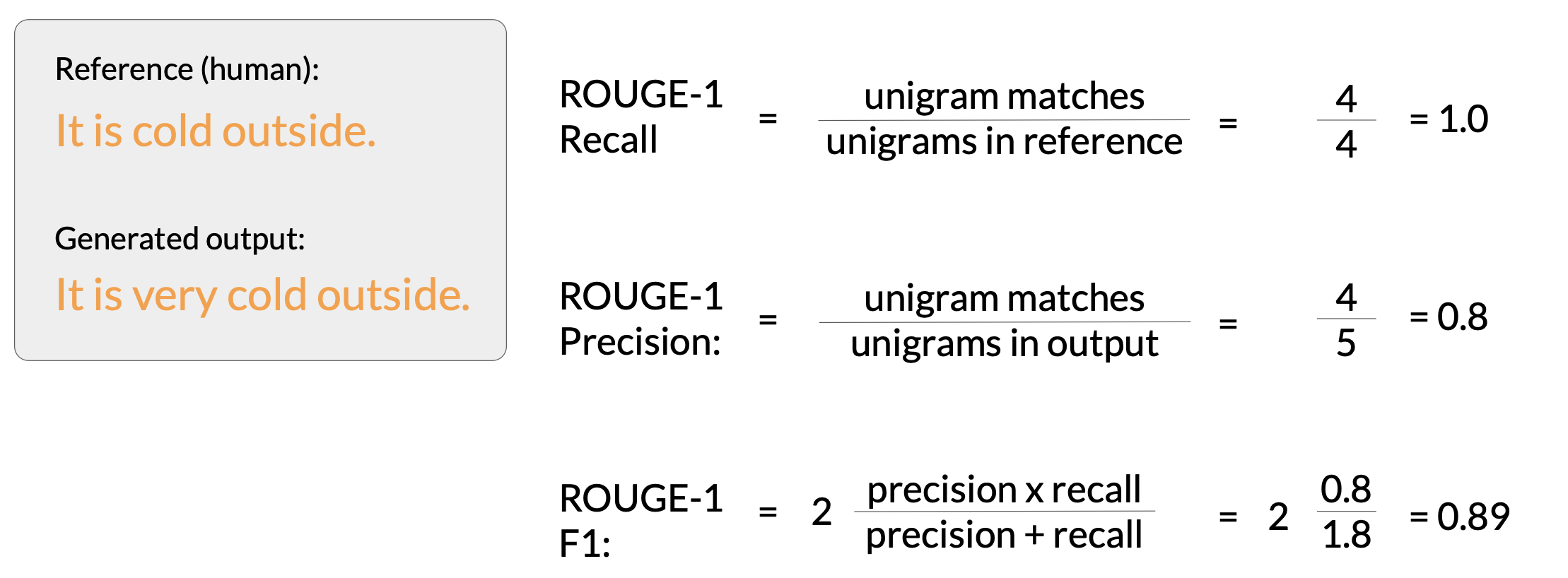
The recall metric measures the number of words or unigrams that are matched between the reference and the generated output divided by the number of words or unigrams in the reference.
Precision measures the unigram matches divided by the output size.
The F1 score is the harmonic mean of both of these values.

Similarly, ROUGE-2, ROUGE-3 simply uses bigram and n-gram to calculate the corresponding results.

ROUGE-L

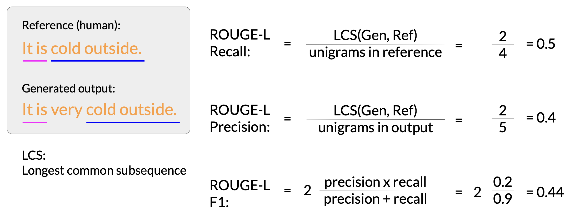
An alternative way is to use the longest common subsequence present in both the generated output and the reference output. In this case, the longest matching sub-sequences are, it is and cold outside, each with a length of two. You can now use the LCS value to calculate the recall precision and F1 score.

BLEU

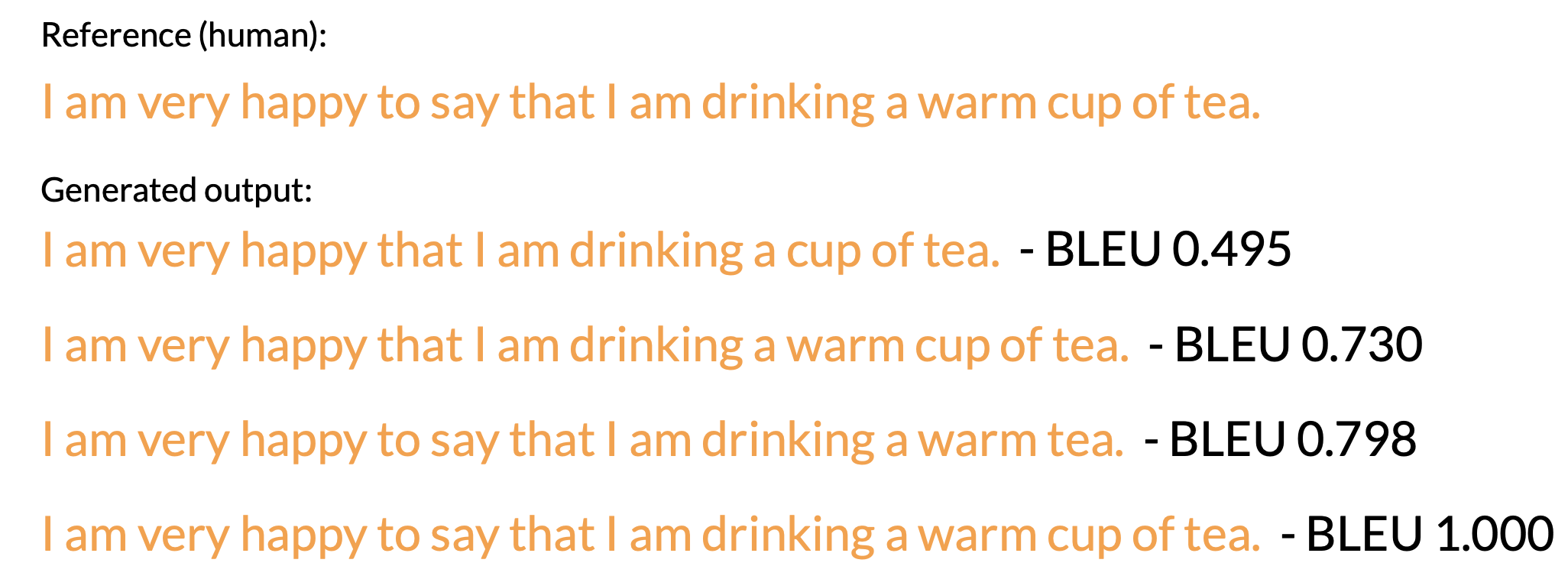
BLEU metric = Avg(precision across range of n-gram sizes)

The BLEU score quantifies the quality of a translation by checking how many n-grams in the machine-generated translation match those in the reference translation. To calculate the score, you average precision across a range of different n-gram sizes.

Benchmarks

As you can see, LLMs are complex, and simple evaluation metrics like the ROUGE and BLEU scores, can only tell you so much about the capabilities of your model.

In order to measure and compare LLMs more holistically, you can make use of pre-existing datasets, and associated benchmarks that have been established by LLM researchers specifically for this purpose.

MMLU (Massive Multitask Language Understanding)

Massive Multitask Language Understanding, or MMLU, is designed specifically for modern LLMs. To perform well models must possess extensive world knowledge and problem-solving ability. Models are tested on elementary mathematics, US history, computer science, law, and more. In other words, tasks that extend way beyond basic language understanding

BIG-bench

BIG-bench currently consists of 204 tasks, ranging through linguistics, childhood development, math, common sense reasoning, biology, physics, social bias, software development and more. BIG-bench comes in three different sizes, and part of the reason for this is to keep costs achievable, as running these large benchmarks can incur large inference costs.

HELM (Holistic Evaluation of Language Models)

The HELM framework aims to improve the transparency of models, and to offer guidance on which models perform well for specific tasks. HELM takes a multimetric approach, measuring seven metrics across 16 core scenarios, ensuring that trade-offs between models and metrics are clearly exposed.

Parameter efficient fine-tuning (PEFT)

Full fine-tuning requires memory not just to store the model, but various other parameters that are required during the training process. Even if your computer can hold the model weights, which are now on the order of hundreds of gigabytes for the largest models, you must also be able to allocate memory for optimizer states, gradients, forward activations, and temporary memory throughout the training process. These additional components can be many times larger than the model and can quickly become too large to handle on consumer hardware

In contrast to full fine-tuning where every model weight is updated during supervised learning, parameter efficient fine tuning methods only update a small subset of parameters. Some path techniques freeze most of the model weights and focus on fine tuning a subset of existing model parameters, for example, particular layers or components.

Other techniques don’t touch the original model weights at all, and instead add a small number of new parameters or layers and fine-tune only the new components. With PEFT, most if not all of the LLM weights are kept frozen. As a result, the number of trained parameters is much smaller than the number of parameters in the original LLM.

With PEFT, most if not all of the LLM weights are kept frozen. As a result, the number of trained parameters is much smaller than the number of parameters in the original LLM. In some cases, just 15-20% of the original LLM weights. This makes the memory requirements for training much more manageable. In fact, PEFT can often be performed on a single GPU. And because the original LLM is only slightly modified or left unchanged, PEFT is less prone to the catastrophic forgetting problems of full fine-tuning.

PEFT Trade-offs

Parameter Efficiency
Memory Efficiency
Model Performance
Training Speed
Inference Costs

PEFT methods

Selective
- Select subset of initial LLM params to fine-tune
- You have the option to train only certain components of the model or specific layers, or even individual parameter types.
- Researchers have found that the performance of these methods is mixed and there are significant trade-offs between parameter efficiency and compute efficiency
Reparameterization
- Reparameterize mdoel weights using a low-rank representation
- Reduce the number of parameters to train by creating new low rank transformations of the original network weights
- LoRA
Additive
- Add trainable layers or parameters to model
- Keep all of the original LLM weights frozen and introducing new trainable components
- Adapters
  - add new trainable layers to the architecture of the model, typically inside the encoder or decoder components after the attention or feed-forward layers
- Soft Prompts
  - keep the model architecture fixed and frozen, and focus on manipulating the input to achieve better performance.
  - This can be done by adding trainable parameters to the prompt embeddings or keeping the input fixed and retraining the embedding weights

LoRA (Low-Rank Adaptation of LLM)

LoRA is a strategy that reduces the number of parameters to be trained during fine-tuning by freezing all of the original model parameters and then injecting a pair of rank decomposition matrices alongside the original weights.

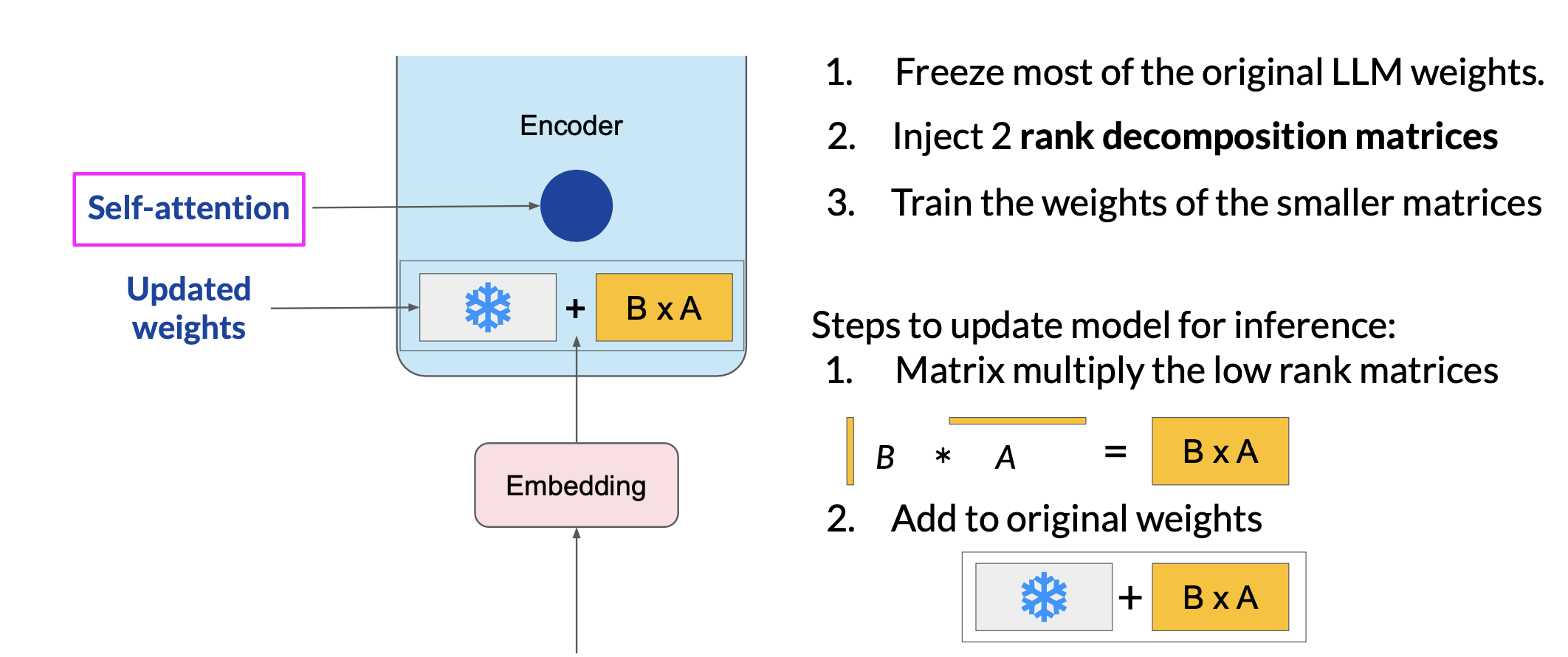
Researchers have found that applying LoRA to just the self-attention layers of the model is often enough to fine-tune for a task and achieve performance gains.

Let’s see a concrete example:

Transformer weights have dimension dxk = 512x64 = 32,768 trainable parameters
In LoRA with rank r=8
- A has dim rxk = 8x64 = 512 params
- B has dim dxr = 512x8 = 4,096 params
- 86% reduction in parameters to train

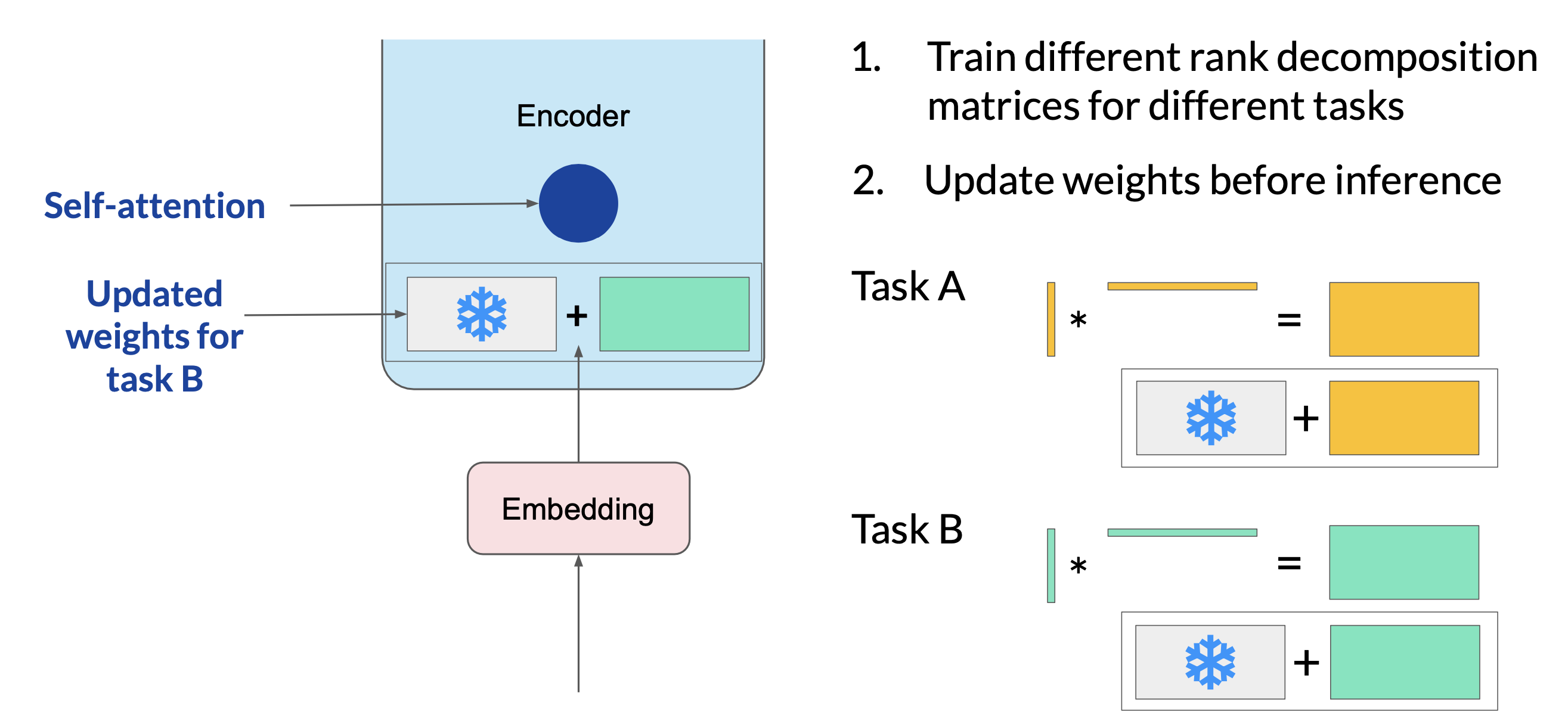
Since the rank-decomposition matrices are small, you can fine-tune a different set for each task and then switch them out at inference time by updating the weights.

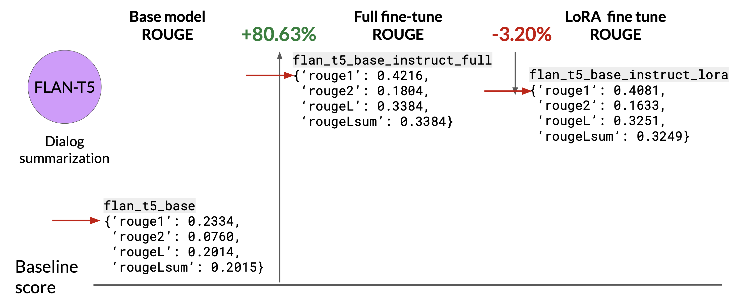
Sample ROUGE metrics for full vs. LoRA fine-tuning

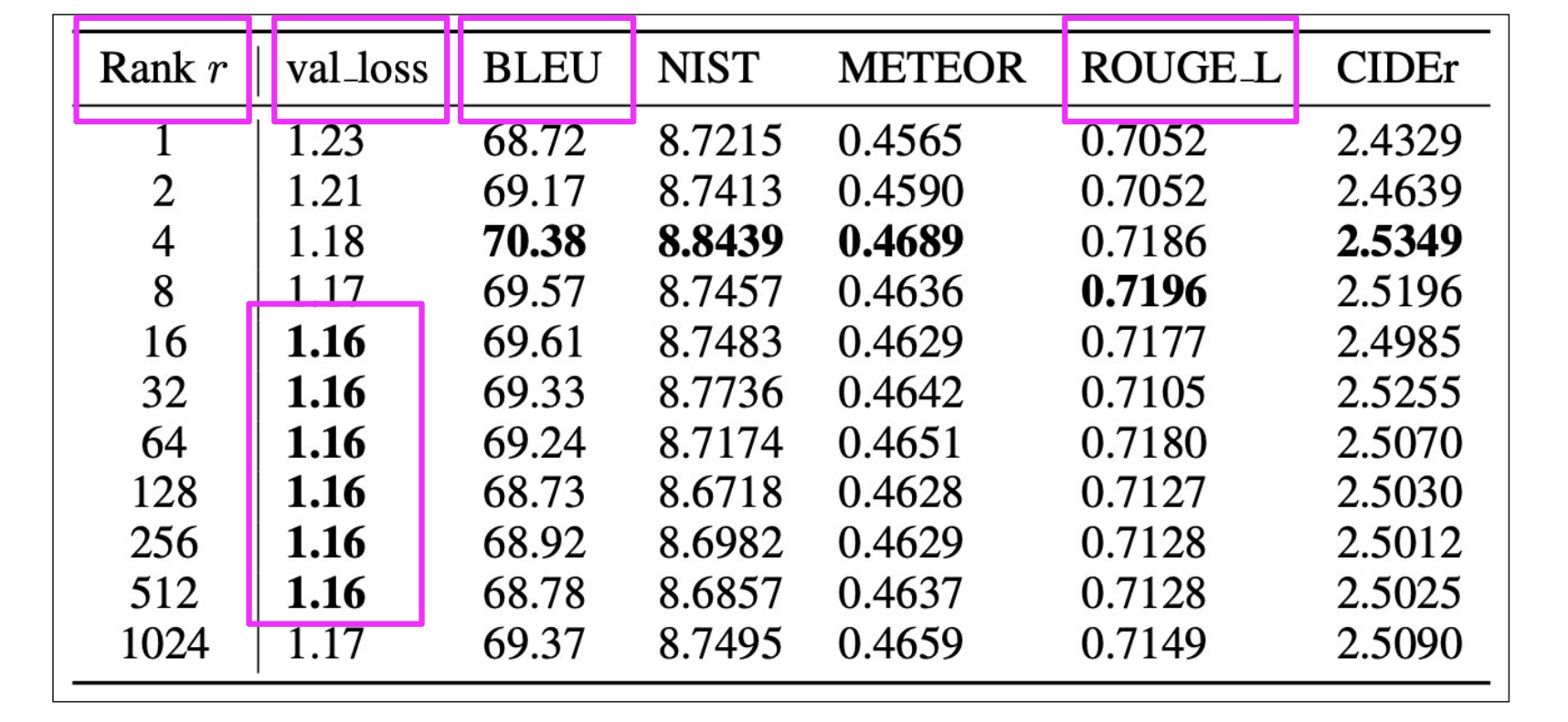
Choose the LoRA rank

Ranks in the range of 4-32 can provide you with a good trade-off between reducing trainable parameters and preserving performance.

Prompt tuning with soft prompts

Prompt tuning is not prompt engineering. With prompt tuning, you add additional trainable tokens to your prompt and leave it up to the supervised learning process to determine their optimal values. The set of trainable tokens is called a soft prompt, and it gets prepended to embedding vectors that represent your input text

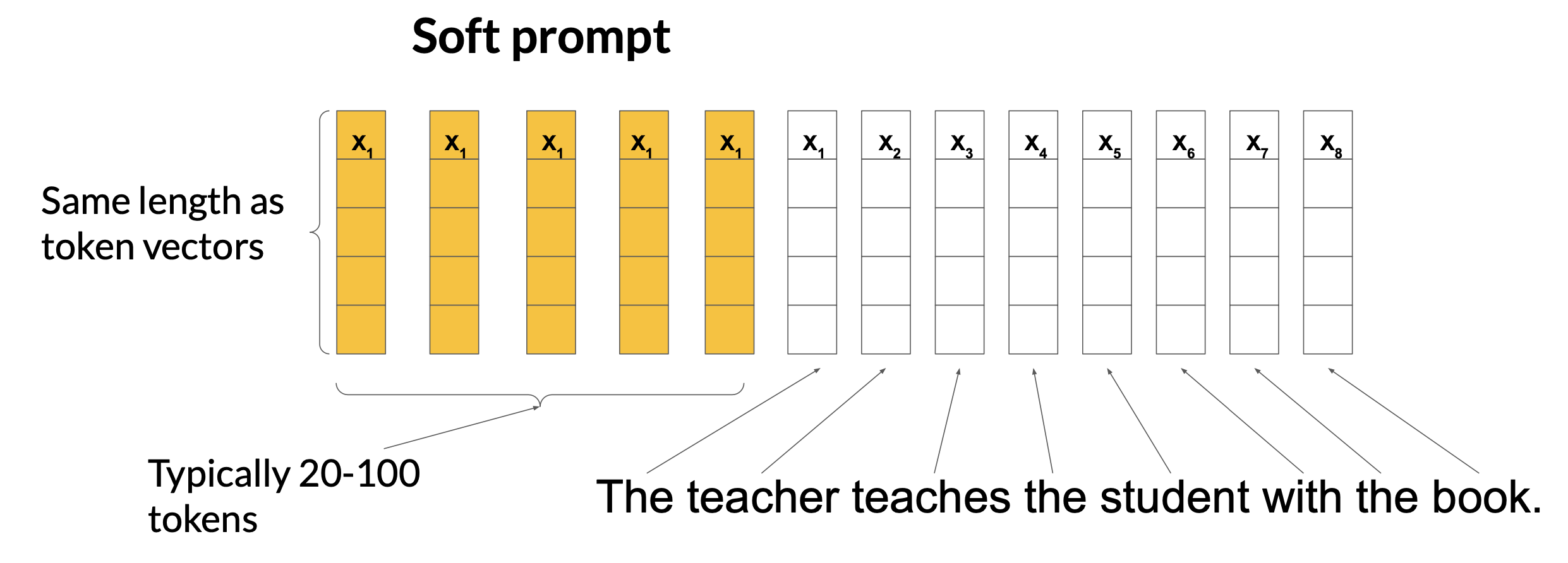
The tokens that represent natural language are hard in the sense that they each correspond to a fixed location in the embedding vector space.

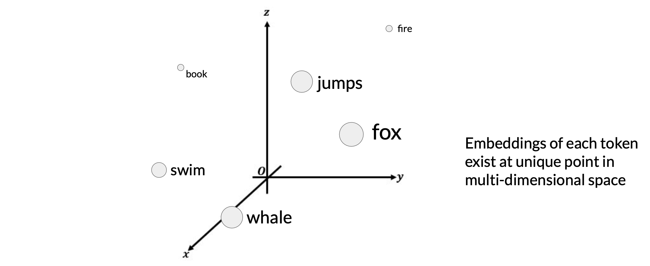
However, the soft prompts are not fixed discrete words of natural language. Instead, you can think of them as virtual tokens that can take on any value within the continuous multidimensional embedding space. And through supervised learning, the model learns the values for these virtual tokens that maximize performance for a given task.

Since the soft prompt tokens can take any value within the continuous embedding vector space. The trained tokens don't correspond to any known token, word, or phrase in the vocabulary of the LLM

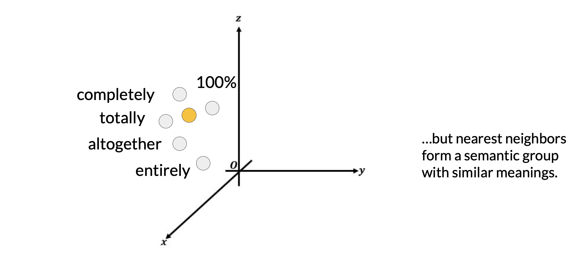
However, an analysis of the nearest neighbor tokens to the soft prompt location shows that they form tight semantic clusters. In other words, the words closest to the soft prompt tokens have similar meanings. The words identified usually have some meaning related to the task, suggesting that the prompts are learning word like representations.

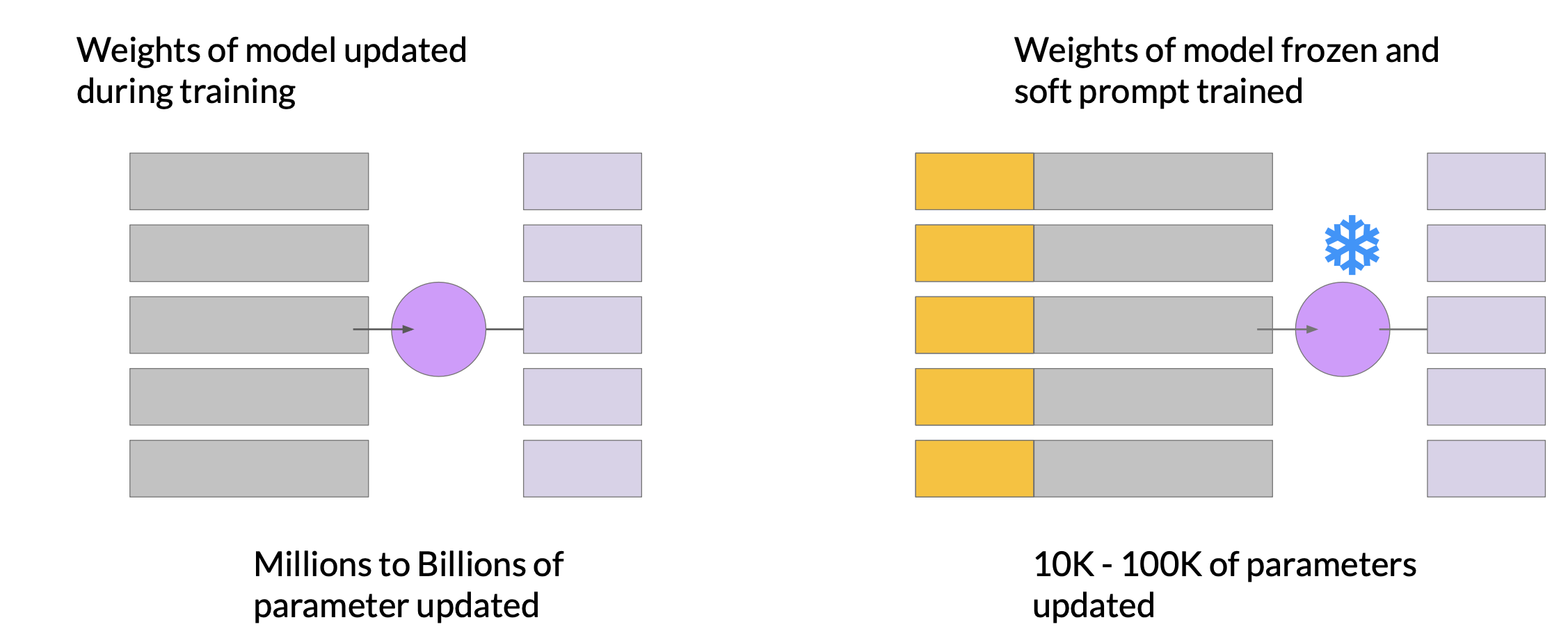
In contrast with prompt tuning, the weights of the large language model are frozen and the underlying model does not get updated. Instead, the embedding vectors of the soft prompt gets updated over time to optimize the model’s completion of the prompt. Prompt tuning is a very parameter efficient strategy because only a few parameters are being trained. In contrast with the millions to billions of parameters in full fine tuning, similar to what you saw with LoRA.

Performance of prompt tuning

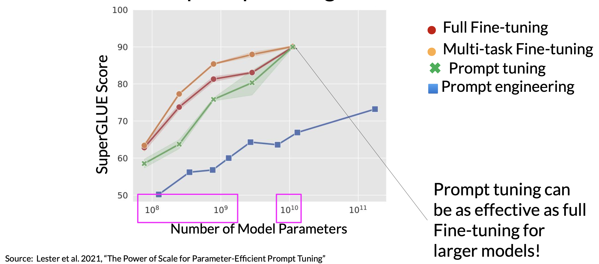
As you can see, prompt tuning doesn’t perform as well as full fine tuning for smaller LLMs. However, as the model size increases, so does the performance of prompt tuning. And once models have around 10 billion parameters, prompt tuning can be as effective as full fine tuning and offers a significant boost in performance over prompt engineering alone.

Resources

Appendix A: Low-Rank Matrix Definition

A matrix A is said to be low-rank if its rank r (the number of linearly independent rows or columns) is much smaller than its dimensions m×n. That is:

\[r \ll \min(m, n)\]

For a low-rank matrix A, we can approximate it using two smaller matrices B and C such that:

\[A \approx BC\]

where:

B is a matrix of size m×r.
C is a matrix of size r×n.