Variational Autoencoder

Variational Autoencoder (VAE)

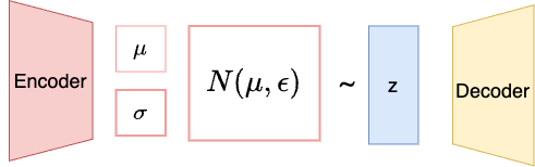
The VAE in Stable Diffusion doesn’t control the image generation process. Instead, it compresses images into a lower-dimensional latent representation before diffusion, and decompresses the final latent back into an image after the diffusion model has finished sampling.

The Autoencoder Architecture

Before we dive into VAEs, it’s important to first understand the architecture of Autoencoder. Autoencoder is a likelihood-based approach for image generation. The Autoencoder architecture consists of three main components: the encoder, the bottleneck(or latent space), and the decoder.

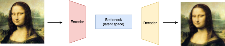
• The encoder compress the input data into a “latent-space” representation, which is a low-dimensional space that captures the essential features of the input data.
• The bottleneck layer is the smallest layer that holds the compressed representation
• The decoder reconstructs the input data from the compressed representation

Training an Autoencoder is a self-supervised process that focuses on minimizing the difference between the original data and its reconstructed version. The goal is to improve the decoder's ability to accurately reconstruct the original data from the compressed latent representation. At the same time, the encoder becomes better at compressing the data in a way of preserving critical information, ensuring that the original data can be effectively reconstructed.

If the model is well-trained, the encoder can be used separately to perform data dimensional reduction. It maps images with similar features (e.g., animals, trees) to nearby regions in latent space. For example, images of dogs will cluster closer to each other than to images of trees in the latent space.

Latent Space

What is latent space, and why is it helpful in Autoencoder or Stable Diffusion?

• Reduced Dimensions: Images in pixel space can be very high-dimensional (e.g., a 512×512 RGB image has 512 × 512 × 3 pixels). Operating in a latent space often reduces the dimensionality by a large factor (e.g., down to 64×64 or 32×32 with several channels), which means fewer computations are required.
• Faster Sampling: The diffusion process, which involves many iterative steps, becomes much faster when each step is operating on a compressed representation.
• Memory Efficiency: Lower-dimensional representations use significantly less memory. This allows for training and sampling on devices with more limited memory (like GPUs) and enables the model to work with larger batch sizes.
• Preserving Semantics: The latent space is designed to capture the high-level, semantic features of an image (like shapes, object positions, and overall style) rather than every fine-grained pixel detail. This focus on semantics allows the diffusion process to operate on the essential content of the image.

Variational Bayes

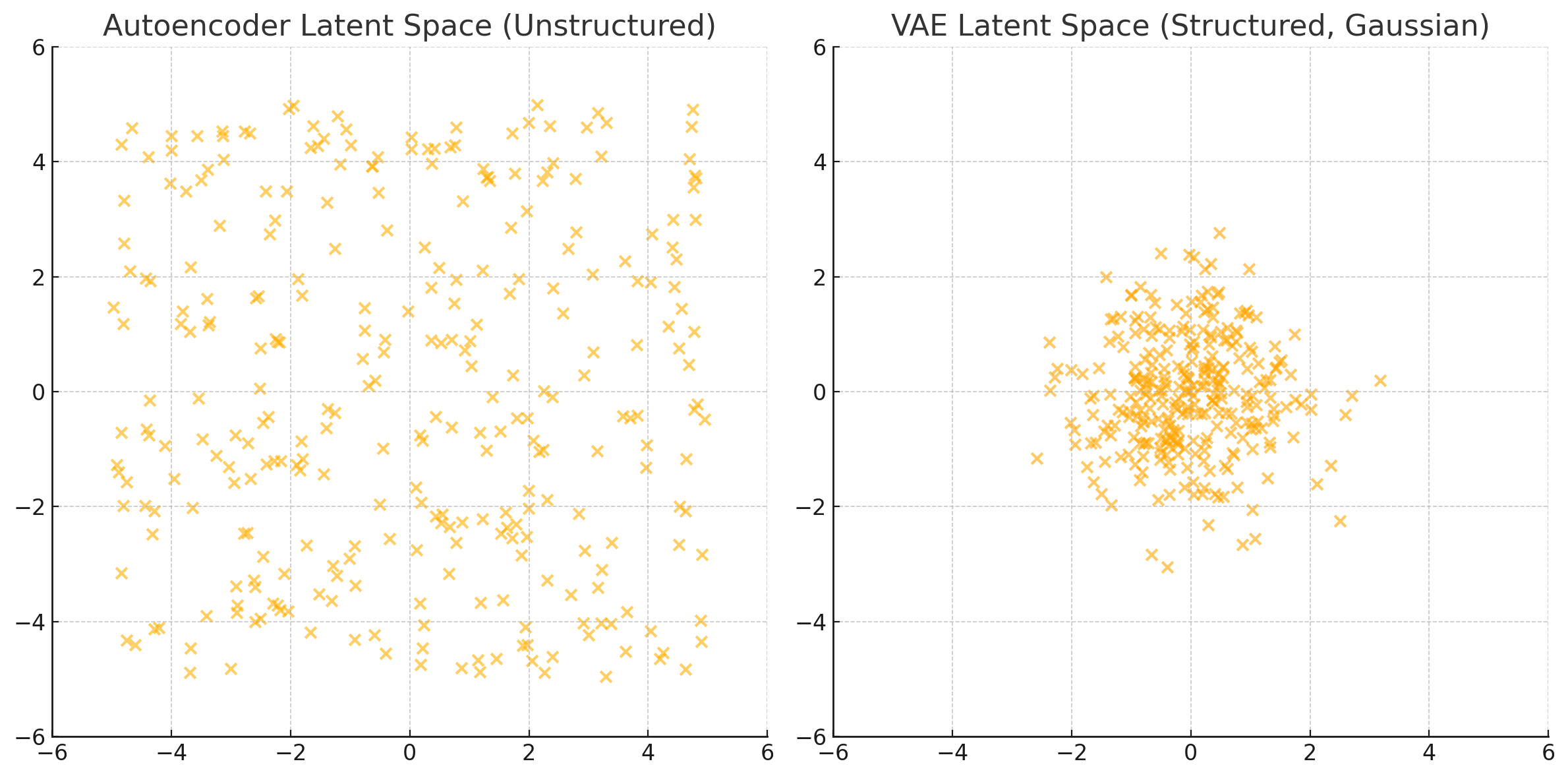
With the Autoencoder architecture, a natural idea for generating new images would be to randomly sample points from this latent space and run them through the decoder. Unfortunately, this approach won’t produce meaningful images mainly because the latent space is unstructured and disorganized. For example, if you sample a random latent vector (say, from $N(0,1)$), there’s no guarantee it maps to a valid image.

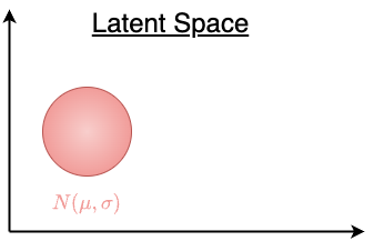
That is why most of modern implementation of Autoencoders regularize the latent space. VAE is the most famous type of regularized autoencoder. The latent space produced by VAE is structured and continuous, following a standard Gaussian distribution. This makes it easy to sample new points and interpolate smoothly between them

VAE was first introduced in 2013 in this paper named Auto-Encoding Variational Bayes. The idea is that, in order to reconstruct an image from a latent vector, we need to calculate the conditional probability $p(x|z)$, where $p(z)$ is a latent distribution that capture the core features of the images. To make this process computable, we assume $p(z)$ follows the standard Gaussian distribution: $p(z) = N(0, 1)$. This allows us to compute the likelyhood $p(x|z)$.

Then the question is how do we produce this Gaussian Distribution? That’s where VAE kicks in, it learns the parameter $\mu$ and $\sigma$, which is an optimization process usually known as variational Bayes. Here is the process:

1. We train a deep encoder to estimate these parameters $\mu$ and $\sigma$ from the images
2. Then we use a decoder to reconstruct images from a sampled latent variable
3. Compare the reconstructed images with the original images with the following loss function:

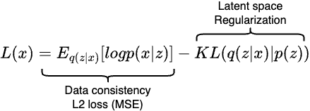
The first part of the equation simply measures how well our model can reconstruct an image $x$ from its encoded latent variable $z$. The $log$ likelyhood term reduces to a simple $L_2$ reconstruction loss, also known as mean square error. It just measures the loss between the reconstructed image and the original image.

The second part of the equation is the KL divergence that measures the distant between two probability distributions. In our case, it measures the distance between $p(z)$ and the normal distribution. While minimizing the loss, $p(z)$ will take shape of the normal distribution as well.

After the training finishes, the latent space should look very closely to the shape of a 2D normal distribution as shown in the image above.

Use VAE to generate images

Once the model is trained, the encoder can encode the images to their latent representation. However, VAE does this a bit differently than the plain Autoencoder. Instead of mapping the input image directly to a single latent vector in the latent space, the VAE encoder converts the input into a group of vectors that follows the Gaussian distribution, namely $\mu$ and $\sigma$. From this latent distribution, we sample points at random, and the decoder converts these sampled points back into the input space. By sampling a random latent vector, we can create a wide variety of new images.

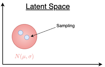
In summary, VAE maintains a compact and smooth latent space, ensuring that most of the points (latent vectors) within the normal distribution in the latent space will lead to plausible samples. Appendix #2 demonstrates how to use VAE in Stable Diffusion 1.5.

Resources

• How Diffusion Models Work
• Denoising Diffusion Probabilities Models
• Using Stable Diffusion with Python

Appendix: VAE in Stable Diffusion

The VAE architecture used in Stable Diffusion 1.5 can be found here. The following code shows how to use VAE to encode and decode an image:

# Encoding

# the image has to conform to the shape of (N,C,H,W)
print(image.shape) # [1, 3, 300, 300]

vae_model = AutoencoderKL.from_pretrained(
    "runwayml/stable-diffusion-v1-5",
    subfolder = "vae",
    torch_dtype=torch.float16,
    cached_dir = CACHE_DIR
)

# encode the image into a laten distribution and sample it randomly
latents = vae_model.encode(image).latent_dist.sample()
print(latents[0].shape) #[4, 37, 37]

# Decoding

with torch.no_grad():
    decode_image = vae_model.decode(
        latents,
        return_dict = False
    )[0][0].to("cpu")

# from [-1, 1] to [0, 1]
decode_image = (decode_image / 2 + 0.5).clamp(0, 1)

print(decode_image.shape) # [3, 296, 296]

Let’s first take a look at the encoding process. As mentioned earlier, the output of encoder is a Gaussian distribution. latents = vae_model.encode(image).latent_dist.sample() does three things:

• vae_model.encode(image) returns an object that contains a distribution(DiagonalGaussianDistribution) over latent vectors.
• .latent_dist is an instance of a Gaussian (Normal) distribution, parameterized by $\mu$ and $\sigma$
• sample() draws a random sample from this distribution

The DiagonalGaussianDistribution is defined as follows:

class DiagonalGaussianDistribution:
    def __init__(self, parameters):
        self.mean, self.logvar = torch.chunk(parameters, 2, dim=1)
        self.std = torch.exp(0.5 * self.logvar)
    
    def sample(self):
        noise = torch.randn_like(self.mean)
        return self.mean + self.std * noise

The shape of encoded latent vector is [4, 37, 37]. This is because

• 4 is latent channels (Stable Diffusion uses 4D latent space instead of RGB’s 3)
• 37x37 is the spatial resolution (input image was 300x300).

How is 37 calculated?

If we examine the VAE architecture, the output of the encoder in our example from this layer:

(conv_out): Conv2d(512, 8, kernel_size=(3, 3), stride=(1, 1), padding=(1, 1))

Since we have three conv2d layers in the encoder, each layer does a stride=1 convolution, thus the size of the image shrinks by half after each layer: 300 -> 150 -> 75 -> 37

Let’s say the output of the conv_out layer is a [1, 8, H, W] latent vector, the next thing we do is to split this tensor to two [1, 4, H, W] tensors for $\mu$ and $\sigma$ respectively:

mu, logvar = torch.chunk(tensor, 2, dim=1)
mu # [1, 4, H, W]
logvar #[1,4, H, W]

Then we do the sampling using $\mu$ and $\sigma$:

std = torch.exp(0.5 * logvar)              # [1, 4, H, W]
eps = torch.randn_like(std)               # [1, 4, H, W]
z = mu + std * eps                        # [1, 4, H, W]

Finally, z is the latent vector that gets passed to the denoising U-Net.