CLIP Encoders

CLIP (Contrastive Language-Image Pre-training)

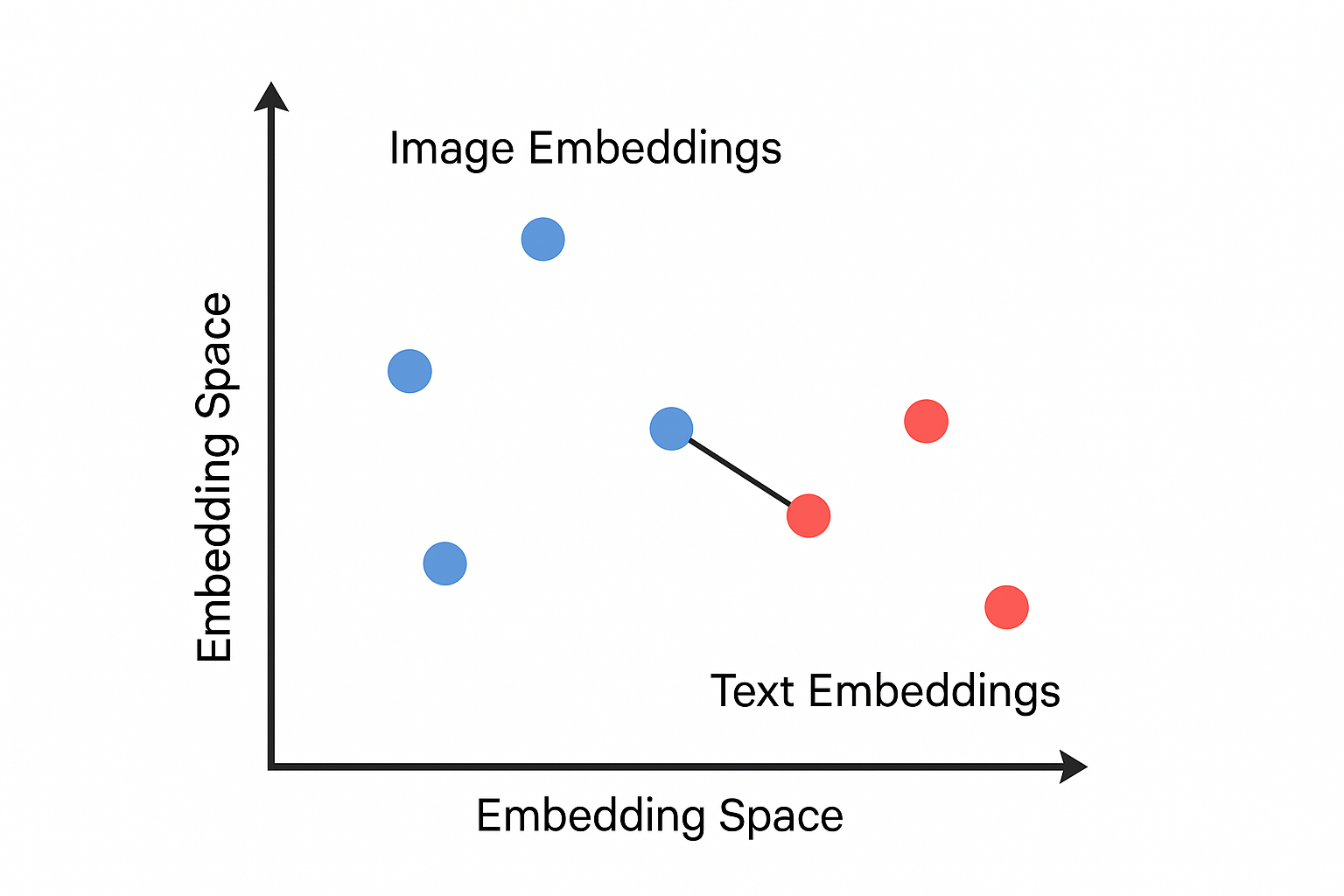
Contrastive learning is a family of self-supervised learning methods that help models learn meaningful representations from data that don’t have labels. The key idea is images that show similar objects should have similar representations

CLIP is one of the Contrastive models. It was first introduced by openAI. The goal is to learn a shared embedding space where text descriptions and images are mapped to vectors that are semantically aligned.

The CLIP model is trained using 400 million (image, text) pairs, where the text is the caption of the image. Thus, after training, the model can encode images and text into a vector that can best represent the images’ content in the CLIP embedding space.

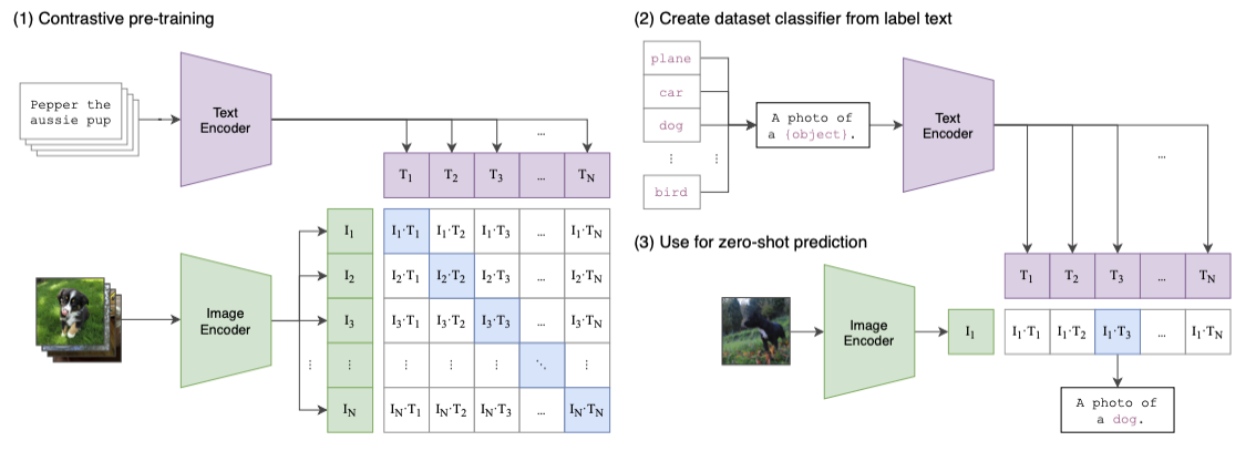
Here is the high-level steps of the training process:

1. Let a batch of images goes through an image encoder(a ResNet50/ViT model) to produce the feature embeddings $I_e$.
2. Let a batch of the corresponding text caption go through a text encoder(a Transformer model) to produce the text embedding $T_e$.
3. Calculate the embedding cosine similarities between $I_e$ and $T_e$
4. Update both encoders’ weights to maximize the similarity for the correct pairs (the blue squares along the diagonal direction in the diagram)
5. Update both encoders’ weights to minimize the similarity for the incorrect pairs (white squares in the diagram)

Once the model is pre-trained, it proceeds through a zero-shot transfer learning phase. Due to length of this post, we won’t cover it in detail here—refer to the original CLIP paper for a thorough explanation.

In Stable Diffusion, only the CLIP text encoder is used to convert text prompts into embeddings. These text embeddings then condition the image generation process. Let’s take a look at one example:

prompt = "a running dog"

# convert prompt to tokens
input_tokens = clip_tokenizer(
    prompt,
    return_tensors = "pt"
)["input_ids"]

print(input_tokens) # [49406, 320, 2761, 7251, 49407]

clip_text_encoder = CLIPTextModel.from_pretrained(
    "runwayml/stable-diffusion-v1-5",
    subfolder = "text_encoder",
    cache_dir=CACHE_DIR
)

# encode input_tokens to embeddings
text_embeds = clip_text_encoder(input_tokens)[0]

# each input token is encoded into a 768-dim vector
print(text_embeds) # ([1, 5, 768])

For Stable Diffusion 1.5, each token will be encoded as a 768 dimensional vector in the CLIP embedding space. They will be used later in the downstream of the network.

Resources

• High-Resolution Image Synthesis with Latent Diffusion Models
• CLIP
• Contrastive Learning
• Auto-Encoding Variational Bayes
• Variational Autoencoders | Generative AI Animated
• Using Stable Diffusion with Python

Appendix #1: CLIP text encoder model architecture

CLIPTextModel(
  (text_model): CLIPTextTransformer(
    (embeddings): CLIPTextEmbeddings(
      (token_embedding): Embedding(49408, 768)
      (position_embedding): Embedding(77, 768)
    )
    (encoder): CLIPEncoder(
      (layers): ModuleList(
        (0-11): 12 x CLIPEncoderLayer(
          (self_attn): CLIPSdpaAttention(
            (k_proj): Linear(in_features=768, out_features=768, bias=True)
            (v_proj): Linear(in_features=768, out_features=768, bias=True)
            (q_proj): Linear(in_features=768, out_features=768, bias=True)
            (out_proj): Linear(in_features=768, out_features=768, bias=True)
          )
          (layer_norm1): LayerNorm((768,), eps=1e-05, elementwise_affine=True)
          (mlp): CLIPMLP(
            (activation_fn): QuickGELUActivation()
            (fc1): Linear(in_features=768, out_features=3072, bias=True)
            (fc2): Linear(in_features=3072, out_features=768, bias=True)
          )
          (layer_norm2): LayerNorm((768,), eps=1e-05, elementwise_affine=True)
        )
      )
    )
    (final_layer_norm): LayerNorm((768,), eps=1e-05, elementwise_affine=True)
  )
)

Appendix #2: VAE in Stable Diffusion

The VAE architecture used in Stable Diffusion 1.5 can be found here. The following code shows how to use VAE to encode and decode an image:

# Encoding

# the image has to conform to the shape of (N,C,H,W)
print(image.shape) # [1, 3, 300, 300]

vae_model = AutoencoderKL.from_pretrained(
    "runwayml/stable-diffusion-v1-5",
    subfolder = "vae",
    torch_dtype=torch.float16,
    cached_dir = CACHE_DIR
)

# encode the image into a laten distribution and sample it randomly
latents = vae_model.encode(image).latent_dist.sample()
print(latents[0].shape) #[4, 37, 37]

# Decoding

with torch.no_grad():
    decode_image = vae_model.decode(
        latents,
        return_dict = False
    )[0][0].to("cpu")

# from [-1, 1] to [0, 1]
decode_image = (decode_image / 2 + 0.5).clamp(0, 1)

print(decode_image.shape) # [3, 296, 296]

Let’s first take a look at the encoding process. As mentioned earlier, the output of encoder is a Gaussian distribution. latents = vae_model.encode(image).latent_dist.sample() does three things:

• vae_model.encode(image) returns an object that contains a distribution(DiagonalGaussianDistribution) over latent vectors.
• .latent_dist is an instance of a Gaussian (Normal) distribution, parameterized by $\mu$ and $\sigma$
• sample() draws a random sample from this distribution

The DiagonalGaussianDistribution is defined as follows:

class DiagonalGaussianDistribution:
    def __init__(self, parameters):
        self.mean, self.logvar = torch.chunk(parameters, 2, dim=1)
        self.std = torch.exp(0.5 * self.logvar)
    
    def sample(self):
        noise = torch.randn_like(self.mean)
        return self.mean + self.std * noise

The shape of encoded latent vector is [4, 37, 37]. This is because

• 4 is latent channels (Stable Diffusion uses 4D latent space instead of RGB’s 3)
• 37x37 is the spatial resolution (input image was 300x300).

How is 37 calculated?

If we examine the VAE architecture, the output of the encoder in our example from this layer:

(conv_out): Conv2d(512, 8, kernel_size=(3, 3), stride=(1, 1), padding=(1, 1))

Since we have three conv2d layers in the encoder, each layer does a stride=1 convolution, thus the size of the image shrinks by half after each layer: 300 -> 150 -> 75 -> 37

Let’s say the output of the conv_out layer is a [1, 8, H, W] latent vector, the next thing we do is to split this tensor to two [1, 4, H, W] tensors for $\mu$ and $\sigma$ respectively:

mu, logvar = torch.chunk(tensor, 2, dim=1)
mu # [1, 4, H, W]
logvar #[1,4, H, W]

Then we do the sampling using $\mu$ and $\sigma$:

std = torch.exp(0.5 * logvar)              # [1, 4, H, W]
eps = torch.randn_like(std)               # [1, 4, H, W]
z = mu + std * eps                        # [1, 4, H, W]

Finally, z is the latent vector that gets passed to the denoising U-Net.

Appendix #3: Cross Attention U-Net

Below is the architecture of Transformer2DModel, which is heart and soul of the cross-attention U-Net.

(attentions): ModuleList(
    (0-1): 2 x Transformer2DModel(
      (norm): GroupNorm(32, 320, eps=1e-06, affine=True)
      (proj_in): Conv2d(320, 320, kernel_size=(1, 1), stride=(1, 1))
      (transformer_blocks): ModuleList(
        (0): BasicTransformerBlock(
          (norm1): LayerNorm((320,), eps=1e-05, elementwise_affine=True)
          (attn1): Attention(
            (to_q): Linear(in_features=320, out_features=320, bias=False)
            (to_k): Linear(in_features=320, out_features=320, bias=False)
            (to_v): Linear(in_features=320, out_features=320, bias=False)
            (to_out): ModuleList(
              (0): Linear(in_features=320, out_features=320, bias=True)
              (1): Dropout(p=0.0, inplace=False)
            )
          )
          (norm2): LayerNorm((320,), eps=1e-05, elementwise_affine=True)
          (attn2): Attention(
            (to_q): Linear(in_features=320, out_features=320, bias=False)
            (to_k): Linear(in_features=768, out_features=320, bias=False)
            (to_v): Linear(in_features=768, out_features=320, bias=False)
            (to_out): ModuleList(
              (0): Linear(in_features=320, out_features=320, bias=True)
              (1): Dropout(p=0.0, inplace=False)
            )
          )
          (norm3): LayerNorm((320,), eps=1e-05, elementwise_affine=True)
          (ff): FeedForward(
            (net): ModuleList(
              (0): GEGLU(
                (proj): Linear(in_features=320, out_features=2560, bias=True)
              )
              (1): Dropout(p=0.0, inplace=False)
              (2): Linear(in_features=1280, out_features=320, bias=True)
            )
          )
        )
      )
      (proj_out): Conv2d(320, 320, kernel_size=(1, 1), stride=(1, 1))
    )
  )

The PyTorch definition of the model lives in diffusers.

Let’s walk through both attn1 (self-attention) and attn2 (cross-attention) for the input tensor - x = [1, 4, H, W]:

• After conv_in: x becomes [1, 768, H, W]
• After flattening, x becomes [1, H*W, 768]

The Self-Attention model is defined as follows(simplified):

class Attention(nn.Module):
    def __init__(self):
        self.to_q = nn.Linear(768, 768, bias=False)
        self.to_k = nn.Linear(768, 768, bias=False)
        self.to_v = nn.Linear(768, 768 ,bias=False)
        self.to_out = nn.Sequential(nn.Linear(768, 768), nn.Dropout(0.0))

    def forward(self, x, context=None):
        if context is None:
            context = x  # ← this is self-attention!

        q = self.to_q(x)       # [B, HW, C]
        k = self.to_k(context) # [B, HW, C]
        v = self.to_v(context) # [B, HW, C]

        scale = q.shape[-1] ** -0.5
        sim = torch.matmul(q, k.transpose(-1, -2)) * scale  # [B, HW, HW]
        attn = torch.softmax(sim, dim=-1)

        out = torch.matmul(attn, v)  # [B, HW, C]
        out = self.to_out(out)
        return out

In self-attention,

• q, k, v all have the shape [1, HW, 768]
• attn = softmax(q @ kᵀ / √768) → [1, HW, HW]
• output = attn @ v → [1, HW, 768]
• Reshape back to [1, 768, H, W] via .permute(0, 2, 1).view(1, 768, H, W)

The Cross-Attention model is defined as follows(simplified):

class Attention(nn.Module):
    def __init__(self):
        self.to_q = nn.Linear(768, 768, bias=False)
        self.to_k = nn.Linear(768, 320, bias=False)
        self.to_v = nn.Linear(768, 320 ,bias=False)
        self.to_out = nn.Sequential(nn.Linear(768, 768), nn.Dropout(0.0))
        
    def forward(self, x, text_embed, mask=None):
        # Project queries from image features
        q = self.to_q(x)  # shape: [B, HW, C]

        # Project keys and values from text_embed
        k = self.to_k(text_embed)  # [B, T_text, C]
        v = self.to_v(text_embed)  # [B, T_text, C]

        # Scaled dot-product attention
        scale = q.shape[-1] ** -0.5
        sim = torch.matmul(q, k.transpose(-1, -2)) * scale  # [B, HW, T_text]

        if mask is not None:
            sim = sim.masked_fill(mask, -float("inf"))

        attn = torch.softmax(sim, dim=-1)  # attention weights
        out = torch.matmul(attn, v)        # [B, HW, C]

        out = self.to_out(out)             # final projection
        return out

Continuing from attn1,

• The input latent vector has shape: [1, 768, H, W] → flattened to [1, HW, 768]
• Text embedding (CLIP) has shape: [1, N, 768] (N tokens, N <= 77)
• q = to_q(x) → [1, HW, 768] from the image latent, where HW = H × W (e.g. 37×37 = 1369)
• k = to_k(text_embed) → [1, N, 768] from the text embeddings, projected to match inner dimension
• v = to_v(text_embed) → [1, N, 768] also from the text embeddings
• attn = softmax(q @ kᵀ / √768) → [1, HW, N] Each image patch (query) attends over N tokens (text prompt length)
• output = attn @ v → [1, HW, 768] Injects textual semantic information into each image patch
• Reshape back to [1, 768, H, W] via: .permute(0, 2, 1).view(1, 768, H, W)