How Stable Diffusion Model Works

Posted on 2025-01-20 | In GenAI , Stable Diffusion

Introduction

In the previous post, we explored the theory behind diffusion models. While the original diffusion model serves as more of a proof of concept, it highlights the immense potential of multi-step diffusion models compared to one-pass neural networks. However, it comes with a significant drawback: the pre-trained model operates in pixel space, which is computationally intensive. In 2022, researchers introduced Latent Diffusion Models, which effectively addressed the performance limitations of earlier diffusion models. This approach later became widely known as Stable Diffusion.

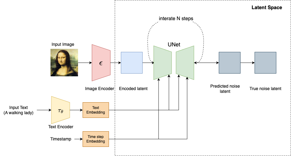
At its core, Stable Diffusion is a collection of models that work together to generate images. These components include:

Tokenizer: Converts a text prompt into a sequence of tokens.
Text Encoder: A specialized Transformer-based language model, specifically the text encoder from a CLIP model.
Variational Autoencoder (VAE): Encodes images into a latent space and reconstructs them back into images.
UNet: The core of the denoising process. This architecture models the noise removal steps by taking inputs such as noise, time-step data, and a conditional signal (e.g., a text representation). It then predicts noise residuals, which guide the image reconstruction process. This combination of components allows Stable Diffusion to efficiently generate high-quality images while significantly reducing computational costs.

Latent Space

Stable Diffusion is a type of latent diffusion model, which means that instead of operating directly in pixel space, it works in a lower-dimensional, compressed representation called the latent space. But why does Stable Diffusion operate in the latent space?

Computational Efficiency
- Reduced Dimensions: Images in pixel space can be very high-dimensional (e.g., a 512×512 RGB image has 512 × 512 × 3 pixels). Operating in a latent space often reduces the dimensionality by a large factor (e.g., down to 64×64 or 32×32 with several channels), which means fewer computations are required.
- Faster Sampling: The diffusion process, which involves many iterative steps, becomes much faster when each step is operating on a compressed representation.
- Memory Efficiency: Lower-dimensional representations use significantly less memory. This allows for training and sampling on devices with more limited memory (like GPUs) and enables the model to work with larger batch sizes.
Preserving Semantics:
- The latent space is designed to capture the high-level, semantic features of an image (like shapes, object positions, and overall style) rather than every fine-grained pixel detail. This focus on semantics allows the diffusion process to operate on the essential content of the image.
- When the model denoises or generates images in this space, it can later decode the latent representations into detailed images via the decoder, which restores the high-resolution details.

Both training and sampling processes happen in the latent space, as shown below

An autoencoder (VAE) is typically used to learn this latent representation. The autoencoder consists of:

Encoder: Compresses the high-dimensional image into a lower-dimensional latent code.
Decoder: Reconstructs the original image from the latent code.

The Inference Process

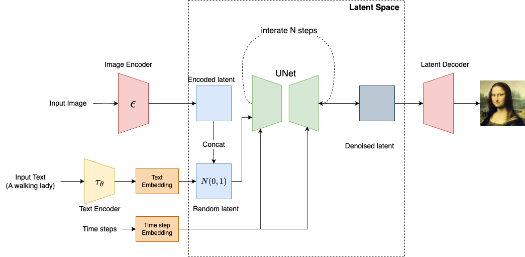
Note that the Stable Diffusion models not only support generating images via prompts, they also support image-guided generation. In the previous article, we start the inference process using a noise image that follows the Gaussian distribution. Here, if text is the only input to the model, we can directly create a noise tensor (e.g., [1, 4, 64, 64]) as the input latent vector.

Stable Diffusion uses CLIP to generate an embedding vector, which will be fed into UNet, using the attention mechanism
If the input contains an image as a guiding signal. The image needs to be first encode to a latent vector and then concat with the randomly generated noise tensor.

The inference process is similar to the training process. After a number of denoting steps, the latent decoder (VAE) converts the image from latent space to the pixel space.

The Stable Diffusion XL (SDXL) model pipeline

SDXL is a latent diffusion model that has the same overall architecture used in Stable Diffusion v1.5. The UNet backbone is three times larger, there are two text encoders in the SDXL base model, and a separate diffusion-based refinement model is included. The overall architecture is shown as follows:

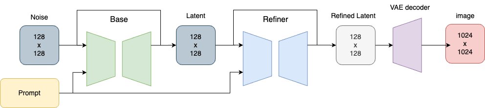
Note that the refiner module is optional. Now let’s break down the components in detail.

The VAE of the SDXL

The VAE used in SDXL is a retrained one, using the same autoencoder architecture but with an increased batch size (256 vs 9). Additionally, it tracks the weights with an exponential moving average. The new VAE outperforms the original model in all evaluated metrics. Here is the code for encoding and decoding an image using VAE:

# encode the image from pixel space to latent space
vae_model = AutoencoderKL.from_pretrained(
    "stabilityai/stable-diffusion-xl-base-1.0",
    subfolder = "vae",
    torch_dtype=torch.float32 # for mps, the fp16 does not work
).to("mps")

image_path = './mona.jpg' 
image = load_image(image_path)

image_processor = VaeImageProcessor()

"""
Converts the image to a normailzed torch tensor in range: [-1, 1]
"""
prep_image = image_processor.preprocess(image)
prep_image = prep_image.to("mps", dtype=torch.float32)
print(prep_image.shape) #[1, 3, 296, 296]
with torch.no_grad():
    image_latent = vae_model.encode(prep_image).latent_dist.sample()

print(image_latent.shape) #[1, 4, 37, 37]

# decode the latent
with torch.no_grad():
    decoded_image = vae_model.decode(image_latent, return_dict = False)[0]
    decoded_image = decoded_image.to("cpu")
   
pil_img = image_processor.postprocess(image = decoded_image, output_type="pil")
pil_img = pil_img[0]
plt.imshow(pil_img)
plt.title("")
plt.axis('off')
plt.show()

Note that a [1, 3, 296, 296] image is encoded into a smaller [1, 4, 37, 37] vector. Additionally, the preprocess will resize the image, such that H/8 and W/8 becomes an integer (296 / 8 = 37).

The UNet of SDXL

UNet is the backbone of SDXL. The UNet backbone in SDXL is almost three times larger, which 2.6G billion trained parameters, while the SD v1.5 has only 860 million parameters. For SDXL, the minimum 15GB of VRAM is the commonly required; otherwise, we’ll need to reduce the image resolution.

Additionally, the SDXL integrates Transformer block within the UNet architecture, making it more expressive and capable of understanding complex text-image relationships. The U-Net still has CNNs, but each downsampled feature map passes through a Transformer-based attention module before being processed further.

Check out this gist to view the SDXL’s unet architecture

Text Encoders

One of the most significant changes in SDXL is the text encoder. SDXL uses two text encoders together, CLIP ViT-L and OpenCLIP Vit-bigG(aka openCLIP G/14).

The OpenCLIP ViT-bigG model is the largest and the best OpenClip model trained on the LAION-2B dataset, a 100 TB dataset containing 2 billion images. While the OpenAI CLIP model generates a 768 dimensional embedding vector, OpenClip G14 outputs a 1,280-dimensional embedding. By concatenating the two embeddings(of the same prompt length), a 2048-dimension embedding is output concat. This is much larger than previous 768-dimensional embedding from Stable Diffusion v1.5.

import torch
from transformers import CLIPTokenizer, CLIPTextModel

prmpt = "a running dog"

clip_tokenizer = CLIPTokenizer.from_pretrained(
    "stabilityai/stable-diffusion-xl-base-1.0",
    subfolder = "tokenizer",
    dtype = torch.float16
)

input_tokens = clip_tokenizer_1(
    prmpt,
    return_tensors = "pt"
)["input_ids"]

print(input_tokens_1) # [49406, 320, 2761, 7251, 49407]

We extract the token_ids from our prompt, resulting in a [1, 5] tensor. Note that 49406 and 49407 represent the beginning and ending symbols, respectively.

clip_text_encoder_1 = CLIPTextModel.from_pretrained(
    "stabilityai/stable-diffusion-xl-base-1.0",
    subfolder = "text_encoder",
).to("mps")

# OpenCLIP ViT-bigG
clip_text_encoder_2 = CLIPTextModel.from_pretrained(
    "stabilityai/stable-diffusion-xl-base-1.0",
    subfolder = "text_encoder_2",
).to("mps")

# encode token ids to embeddings
with torch.no_grad():
    prompt_embed_1 = clip_text_encode_1(
        input_tokens_1.to("mps")
    )[0]
    print(prompt_embed_1.shape) #[1, 5, 768]
    prompt_embed_2 = clip_text_encoder_2(
        input_tokens_2.to("mps")
    )[0]
    print(prompt_embed_1.shape) #[1, 5, 1280]

prompt_embedding = torch.cat((prompt_embed_1, prompt_embed_2), dim = 2) ##[1, 5, 2048]

The code above produces an embedding vector with the shape [1, 5, 768], which is expected because it transforms one-dimensional token IDs into 768-dimensional vectors. We then switch to the OpenCLIP ViT-bigG encoder to encode the same input tokens, resulting a [1, 5, 1280] embedding tenor. Finally, we concatenate these two tensors as the final embedding.

In real world, SDXL uses something called pooled embeddings from OpenCLIP ViT-bigG. Embedding pooling is the process of converting a sequence of tokens into one embedding vector. In other words, pooling embedding is a lossy compression of information.

Unlike the embedding in the above python example, which encodes each token into an embedding vector, a pooled embedding is one vector that represents the whole input text.

# pooled embedding
clip_text_encoder_3 = CLIPTextModelWithProjection.from_pretrained(
    "stabilityai/stable-diffusion-xl-base-1.0",
    subfolder = "text_encoder_2",
    torch_dtype = torch.float16
).to("mps")

# encode token ids to embeddings
with torch.no_grad():
    prompt_embed_3 = clip_text_encoder_3(
        input_tokens_1.to("mps")
    )[0]
print(prompt_embed_3.shape)

The encoder will produce a [1, 1280] embedding tensor, as the maximum token size for a pooled embedding is 77. In SDXL, the pooled embedding is provided to the UNet together with the token-level embedding from both CLIP and OpenCLIP encoders.

The two-stage design

The refiner model is just another image-to-image model used to enhance an image by quality adding more details, especially during the last 10 steps. It may not be necessary if the base model can already produce high quality images.

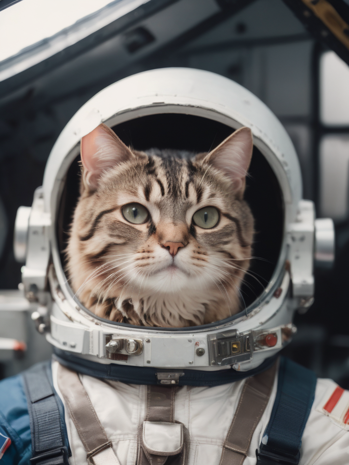
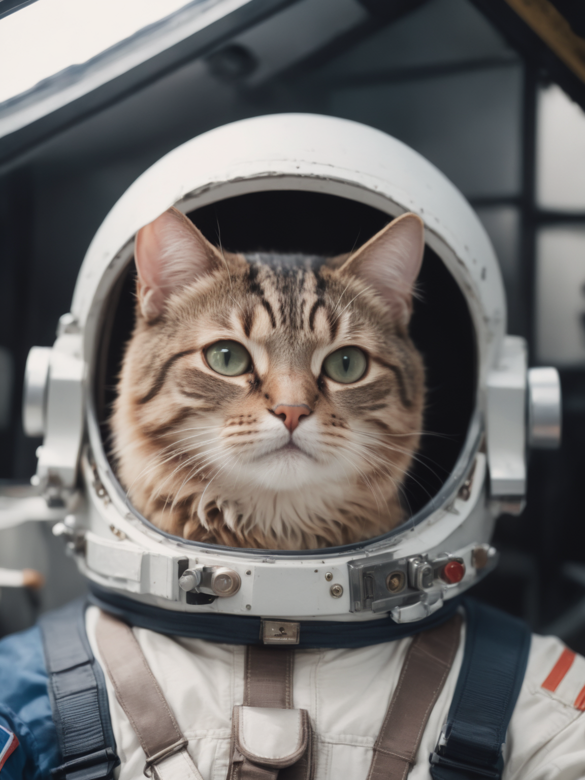
The photo on the left was created using the SDXL base model, while the one on the right was enhanced by a refined model based on the original. At first glance, the differences may be subtle, upon a closer look, you will notice more details (the cat’s hair) were added by the refine model to make the image appear more realistic.

Use Stable Diffusion

Generation Seed

A seed is a random number that is used to control the image generation. It is utilized to generate a noise tensor, which the diffusion model then employs to create an image. When the same seed is used with identical prompts and settings, it typically results in the same image being produced.

Reproducibility: Utilizing the same seed ensures that you can reliably generate the same image when using identical settings and prompts.
Exploration: By changing the seed number, you can explore a wide range of image variations, often leading to the discovery of unique and fascinating results.

If no seed is provided, the Diffuser package will automatically generate a random number for each image generation process.

seed = 1234
generator = torch.Generator("mps").manual_seed(seed)
prompt = "a flying cat"
image = sd_pipe(
    prompt = prompt,
    generator = generator
)

Sampling Scheduler

In the previous post, the sampling (denoise) process usually requires 1,000 steps to finish. To shorten the process, the scheduler allows us to generate images in as few as 20 to 50 steps

from diffusers import EulerDiscreteScheduler

sd_pipe.scheduer = EulerDiscreteScheduler.from_config(
    sd_pipe.sheduler.config
)
generator = torch.Generator("mps").manual_seed(1234)
prompt = "a flying cat"
image = sd_pipe(
    prompt = prompt,
    generator = generator,
    num_inference_steps = 20
).images[0]

The diffusers package provides multiple scheduler to choose. Each scheduler has advantages and disadvantages. You may need to try out the schedulers to find out which one fits the best.

Guidance scale

Guidance scale or Classifier-Free Guidance(CFG) is a parameter that controls the adherence of the generate image to the text prompt. A higher guidance scale will force the image to be more aligned with the prompt, while a lower guidance scale will give more space for the model to decide what to put into the image.

image = sd_pipe(
    prompt = prompt,
    generator = generator,
    num_inference_steps = 20,
    guidance_scale = 7.5
).images[0]

In practice, besides prompt adherence, a high guidance scale also has the following effects:

Increases the color saturation
Increases the contrast
May lead to a blurred image if set too high

The guidance_scale parameter is typically set between 7 and 8.5. A value of 7.5 is good default value.