Theory Behind the Diffusion Models

Introduction

In previous articles, we have explored an image generation technique using the GAN network. However, in the world of generative models, utilizing diffusion models to generate images has now become a new trend. In Jan 2020, a paper titled Denoising Diffusion Probabilities Models introduced a diffusion-based probability model for image generation. The term diffusion is borrowed from thermodynamics. The original meaning is the movement of particles from a region of high concentration to a region of low concentration.

This idea of diffusion inspired machine learning researchers to apply it to denoising and sampling process. In other words, we can start with a noisy image and gradually transforms an image with high-levels of noise into a clear version of the original image. Therefore, this generative model, is referred to as a denoising diffusion probability model.

In this post, we will explore the theory behind diffusion models and dive deeper into three key processes:

• The image-to-noise transformation
• The noise-to-image reconstruction
• The sampling process

Understanding these concepts will give us a solid foundation to grasp how diffusion models work, paving the way for a deeper dive into Stable Diffusion later on.

The image-to-noise transformation

At a high-level, the image to noise process is quite straightforward:

1. Normalize the pixels in the image so that their values are within the range [-1,1].
2. Generate a noise image of the same size as the original image.
   • The noise should follow a Gaussian distribution (standard normal distribution).
3. Mix the noise image and the original image channel by channel (R, G, B) using the following formula:

where $\epsilon$ represents Gaussian noise, $x$ represents the pixel values of the image, and $\beta$ is a float number between [0,1].

The squares of $\sqrt{\beta}$ and $\sqrt{1 - \beta}$ sum to 1, satisfying the Pythagorean theorem. This means that as $\beta$ changes, the proportion of noise in the original image will also change.

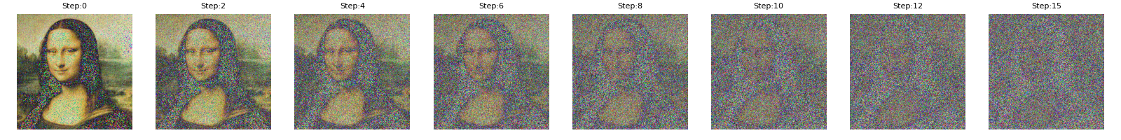
For example, as $\beta$ increases, the proportion of the original image gradually decreases:

It is important to note that each step above relies on the result of the previous calculation. In other words, the noise-adding process is an iterative process, expressed as:

where $\epsilon_t$ follows a standard normal distribution:

Additionally, the value of $\beta_t$ keeps increasing at each step:

Let us define:

Then the above formula can be rewritten as:

Next, we can consider whether it is possible to directly derive $x_t$ from $x_0$, which would eliminate the need for intermediate iterative steps (from $x_1$ to $x_{t-1}$).

It turns out that we can achieve this using the reparameterization trick. By applying mathematical induction (the detailed derivation is omitted here), we can have the following equation:

Here, $\alpha_t \alpha_{t-1} \alpha_{t-2} \alpha_{t-3} \cdots \alpha_2 \alpha_1$ is quite long, so we represent it as $\bar{\alpha}_t$. The equation above can then be further simplified as:

This means that, we can create a list of $\beta_t$, for each moment $t$, we can directly derive $x_t$ from the original image $x_0$. The following code simulates the above process

# --- Step 1: Read and Normalize the Image ---
img_path = './mona.jpg'
img = plt.imread(img_path)

# Normalize: convert from [0, 255] to [0, 1] and then to [-1, 1]
img = img.astype(np.float32) / 255.0
img = img*2 -1 # [0, 1] -> [-1, 1]

# --- Step 2: Set Up the Diffusion Parameters ---
num_iteration = 16
betas = np.linspace(0.0001, 0.02, num_iteration)

alpha_list= [1 - beta for beta in betas ]
# at a given time t,  = a_t * a_{t-1}* ... * a_1
alpha_bar_list = list(accumulate(alpha_list, lambda x, y: x * y))

# --- Step 3: Compute x_t ---
# We'll select timesteps: 0, 2, 4, ..., 14 (total 8 images)
selected_indices = list(range(0, num_iteration, 2))
images = []

for t in selected_indices:
    # Compute the noisy image at timestep t:
    x_t = (np.sqrt(1 - alpha_bar_list[t]) * np.random.normal(0, 1, img.shape) +
                np.sqrt(alpha_bar_list[t]) * img)
    
    # Restore x_t from [-1,1] back to [0,1]
    x_t = (x_t + 1) / 2
    # Convert to uint8 ([0,255]) for display
    x_t = (x_t * 255).astype('uint8')
    images.append(x_t)

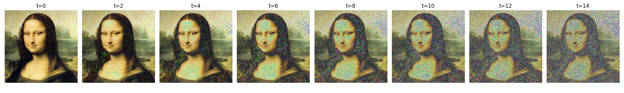
# --- Step 4: Display the 8 Images in One Row ---
show_images()

For simplicity, we perform 16 iterations and select 8 images for display:

The noise-to-image reconstruction

To recover the image from a noise, we need to find the way to recover $x_0$ from $x_t$. However, this revert process is uncomputable without additional information.

From the perspective of probability theory, we aim to compute the conditional probability $p(x_{t-1}|x_t)$. This conditional probability can be described using Bayes’ theorem:

The transition from $x_t$ to $x_{t-1}$ ​is a stochastic process. Substituting it into the Bayes’ formula, we get:

For simplicity, we omit the mathematical derivation. Eventually, we can describe $p(x_{t-1}|x_t)$ using the following formula:

In the previous section, we learned that an image at any time step $x_t$ can be considered as being directly derived from adding noise to an original image $x_0$. As long as we know the noise ϵ added from $x_0$ to $x_t$, we can determine the probability distribution of the previous time step $x_{t-1}$.

Therefore, ϵ is the additional information we're looking for. How to obtain ϵ becomes the next focus in our discussion.

Here, we can train a neural network model that takes the image at time step $x_t$ as input, and predicts the noise ϵ added to this image relative to the original image $x_0$. The predicted the noise should be close to the Gaussian distribution.

Let’s just treat the neural network as a black box for now, and only focus on the input and output of the model. The neural network's output is the noise ϵ, and we compare the predicted noise against the standard Gaussian distribution to calculate the loss:

Why take timestamp $t$ as input? Because all the denoising process share the same neural network weights, the input $t$ will help train a UNet with a time step in mind.

For any normal probability distribution, there are two key parameters: the mean µ and the variance θ. In the original DDRM paper, the model uses a fixed variance, and the mean µ is the only parameter that needs to be learned through a neural network.

At high-level, the training loop can be described like this:

# helper function: perturbs an image to a specified noise level
def perturb_input(x, t, noise):
    return ab_t.sqrt()[t, None, None, None] * x + (1 - ab_t[t, None, None, None]) * noise

for ep in range(n_epoch):
    # code for setup setup learning rate, etc...
    
    # noise is the ϵ ~ N(0,1) with the shape of x_t
    noise = torch.randn_like(x_t)
    # grab the x_t. 
    x_pert = perturb_input(x, t, noise)
    # x_pert is the noised image at step "t"
    pred_noise = nn_model(x_pert, t)
    # loss is mean squared error between the predicted and true noise
    loss = F.mse_loss(pred_noise, noise)
    loss.backward()

The key step here is the perturb_input function. This function produces the noised image at the time step $t$ following the image-to-noise process discussed in the previous section. To recall the process, the code essentially just computes $x_t$ using the following formula:

The sampling process

Once we have this neural network trained, we can start the sampling process to generate our image. At any time step $t$, we can obtain the predicted noise $\epsilon$ from the input noisy image $x_t$. We then pass $\epsilon$ and $x_t$ to a sampling process to produce $x_{t-1}$. Next, we feed $x_{t-1}$ into the model again and repeat this process iteratively until we eventually obtain $x_0$

Note that the very first input to the model (initial $x_t$) can be obtained by simply sampling noise from a Gaussian distribution.

The sampling process can be described using the following steps:

• Generate a complete Gaussian noise with a mean of 0 and a variance of 1. We will use this noise as the starting image:

• Loop through t=T to t=1. In each step, if t>1, then generate another noisy image z (same processing in the image-to-noise section). z also follows the Gaussian distribution:

• Generate a noise from the UNet model, and remove the generated noise from the input noisy image $x_t$:

• Loop end, return the final generated image $x_0$

If we take a look at the previous discussion, all those $\alpha_t$ and $\bar{\alpha_t}$ are known numbers derived from $\beta$. The only thing we need from the UNet is the $\epsilon_\theta(x_t,t)$, which is the noise produced by the UNet.

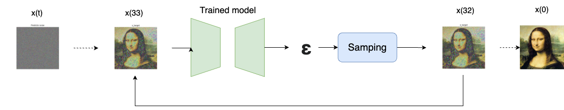
The following diagram illustrates the sampling process:

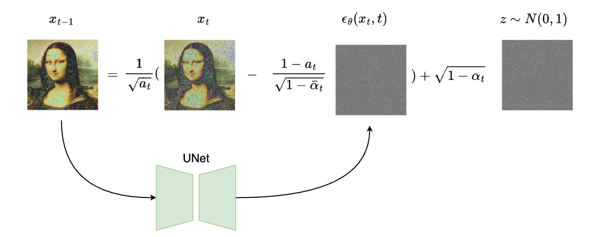
Note that we add a noise($\sqrt{1 - \alpha_t} \times z$) to the end of the formula to stabilize the model. This is found to be useful by searchers that will significantly improve the generated image quality.

PyTorch’s implementation of the sampling process

def denoise_add_noise(x, t, pred_noise, z=None):
    if z is None:
        z = torch.randn_like(x)
    noise = b_t.sqrt()[t] * z
    mean = (x - pred_noise * ((1 - a_t[t]) / (1 - ab_t[t]).sqrt())) / a_t[t].sqrt()
    return mean + noise

def sample_ddpm(n_sample, save_rate=20):
    # x_T ~ N(0, 1), sample initial noise - [N, C, H, W]
    samples = torch.randn(n_sample, 3, height, height).to(device)  

    # array to keep track of generated steps for plotting
    intermediate = [] 
    for i in range(timesteps, 0, -1):
        print(f'sampling timestep {i:3d}', end='\r')

        # reshape time tensor - [N, C, H, W]
        t = torch.tensor([i / timesteps])[:, None, None, None].to(device)

        # sample some random noise to inject back in. For i = 1, don't add back in noise
        z = torch.randn_like(samples) if i > 1 else 0

        eps = nn_model(samples, t)    # predict noise e_(x_t,t)
        samples = denoise_add_noise(samples, i, eps, z)
        if i % save_rate ==0 or i==timesteps or i<8:
            intermediate.append(samples.detach().cpu().numpy())

    intermediate = np.stack(intermediate)
    return samples, intermediate

Resources

• How Diffusion Models Work
• Denoising Diffusion Probabilities Models
• Using Stable Diffusion with Python