Fine-tunning Stable Diffusion Models
LoRA Fine-tuning
In previous articles, we briefly discussed LoRA as a method for fine-tuning LLMs. With LoRA, the original model remains unchanged and frozen, while the fine-tuned weight adjustments are stored separately in what is known as a LoRA file.
LoRA works by creating a small, low-rank model that is adapted for a specific concept. This small model can be merged with the main checkpoint model to generate images during the inference stage.
Let’s use $W$ to represent the original UNet attention weights(Q, K, V), $\Delta W$ to denote the fine-tuned weights from LoRA, and $W’$ as the combined weights. The process of adding LoRA to a model can be expressed as:
If we want to control the scale of LoRA weights, we can leverage a scale factor $\alpha$:
\[W' = W + \alpha\Delta W\]The range of $\alpha$ can be from 0 to 1.0. It should be fine if we set $\alpha$ slightly larger than 1.0.
The reason why LoRA is so small is that $\Delta W$ can be represented by two small low-rank matrices $A$ and $B$, such that:
\[\Delta W = AB^T\]Where $A$ is a n x d matrix, and $B$ is a m x d matrix. For example, if $\Delta W$ is a 6x8 matrix, there a total of 48 weight numbers. Now, in the LoRA file, the 6x8 matrix can be divided by simply two small matrices - a 6x2 matrix, 12 numbers in total, and another 2x8 matrix, making it 16 numbers. The total trained parameters have been reduced from 48 to 28. This is why the LoRA file can be so small.
So, the overall idea of merging LoRA weights to the checkpoint model works like this:
- Find the $A$ and $B$ weight matrices from the LoRA file
- Match the LoRA module layer name to the model’s module layer name so that we know which matrix to patch
- Produce $\Delta W = AB^T$
- Update the model weights
LoRA in practice
To utilize LoRA, we can leverage the load_lora_weights method from StableDiffusionPipeline. The example below demonstrates how to apply two LoRA filters. The adapter_weights parameter determines the extent to which the LoRA model’s “style” influences the output.
# LoRA fine tuning

pipeline.to("mps")

pipeline.load_lora_weights(
    "andrewzhu/MoXinV1",
    weight_name = "MoXinV1.safetensors",
    adapter_name = "MoXinV1",
    cache_dir = cache_dir
)

pipeline.load_lora_weights(
    "andrewzhu/civitai-light-shadow-lora",
    weight_name = "light_and_shadow.safetensors",
    adapter_name = "light_and_shadow",
    cache_dir = cache_dir
)

pipeline.set_adapters(
    ["MoXinV1", "light_and_shadow"],
    adapter_weights = [0.5, 1.0]
)
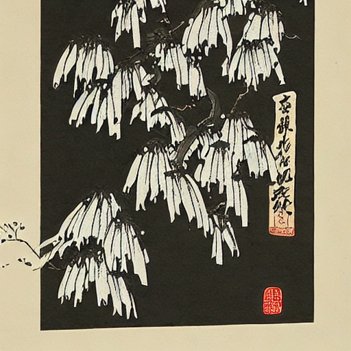
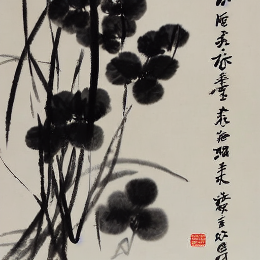
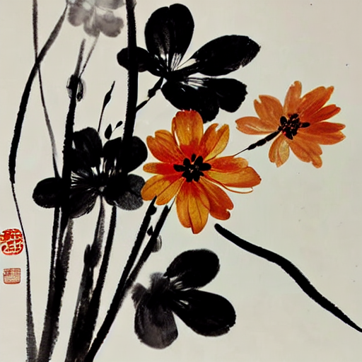
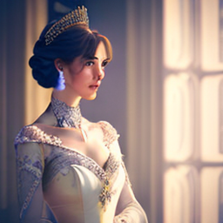
The images below showcase a Chinese painting generated using the Stable Diffusion 1.5 model. The middle image enhances realism, making it look like an authentic Chinese painting. Meanwhile, the second LoRA model introduces more vibrant colors, transforming it into a different artistic style.
Textual Inversion
Textual Inversion(TI) is another way to fine tune the pretrained model. Unlike LoRA, TI is a technique to add new embedding space based on the trained data. Simply put, TI is a text embedding that matches the target image the best, such as its style, object, or face. The key is to find the new embedding that does not exist in the current text encoder.
How does TI works
A latent diffusion model can use images as guidance during training. For training a TI model, we will follow the same pipeline from the previous article, using a minimal set of three to five images, though larger datasets often yield better results.
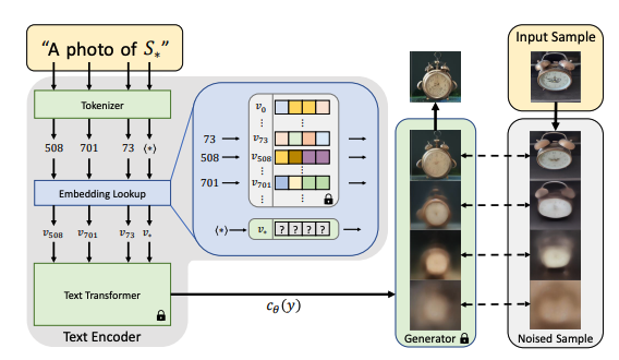
The goal of training is to find a new embedding represented by $v_$. We use $S_$ as the token string placeholder to represent the new concepts we wish to learn. We aim to find a single word embedding, such that sentences of the form “A photo of S*” will lead to the reconstruction of images from our small training set. This embedding is found through an optimization process shown in the above figure, which we refer to as "Textual Inversion".
For example, let’s say we have 5-7 images of a new object, like a custom teddy bear. We want the model to learn what this plush toy looks like. Instead of describing the object in words (e.g., “a teddy bear”), we use S* in the prompt:
- “A photo of S* in a forest”
- “S* sitting on a table”
- “A close-up of S* with soft fur”
Here, S* starts as a meaningless embedding, but during training, it gradually learns the visual characteristics of the teddy bear. After training S* now represents the teddy bear in latent space. You can use it in new prompts:
- “S* in a futuristic city”
- “A cartoon drawing of S*”
- “S* as a superhero”
Now, let talk about the v*. First, recall that the loss function we use to train a latent diffusion model:
The right-hand side is an optimization objective, meaning we are minimizing a loss function, where
- $\epsilon$: The actual noise that was added to the latent representation.
- $\epsilon_{\theta}(z_t, t, c_{\theta}(y))$: The model’s predicted noise at time $t$.
The loss term measures the difference between two noise:
\[\left[ \left\| \epsilon - \epsilon_{\theta}(z_t, t, c_{\theta}(y)) \right\|_2^2 \right]\]So, the right-hand side ensures the model learns to predict the noise accurately, which is key in a diffusion model.
TI reuses the same training scheme as the original LDM model, while keeping both $c_{\theta}$ and $e_{\theta}$ fixed. Our optimization objective is to find the optimal $v_{*}$ that minimizes the loss above.
Since we are learning a new embedding $𝑣_{∗}$, we do not have a predefined text embedding, that’s why the loss function for TI looks like this:
\[v_* = \arg\min_v \mathbb{E}_{z \sim \mathcal{E}(x), y, \epsilon \sim \mathcal{N}(0,1), t} \left[ \left\| \epsilon - \epsilon_{\theta}(z_t, t, c_{\theta}(y)) \right\|_2^2 \right]\]The equation above does not say the embedding equals the loss. Instead, we say
v∗is the embedding that, when used, results in the smallest possible noise prediction loss.
What This Means is that
- Instead of using a fixed text embedding, we introduce $v$, which is a trainable vector.
- We find the best embedding $v_{*}$ that minimizes the LDM loss by optimizing $v$ over multiple training images.
- The
argminnotation means we are searching for the best $v$ that minimizes the noise prediction error.
Once the new corresponding embedding vector is found, the training is done. The output of the training is usually a vector with 768 numbers in the format of pt or bin file. The files are typically just a few kilobytes in size. This makes TI a highly efficient method for incorporating new elements or styles into the image.
For example, the code below loads a TI model(a bin file) from the Hugging Face concepts library. The bin structure is just a key-value pair:
import torch
loaded_leared_embeds = torch.load('/Volumes/ai-1t/ti/midjourney_style.bin', map_location='cpu')
keys = list(loaded_leared_embeds.keys())
for key in keys:
    print(key, ": ", loaded_leared_embeds[key].shape) # <midjourney-style> :  torch.Size([768])
TI in practice
To use TI models, we could just leverage the load_textual_inversion method from the StableDiffusionPipeline
pipe.load_textual_inversion(
    "sd-concepts-library/midjourney-style",
    token = "midjourney-style",
)
This method does two things:
- Registers a New Learnable Token
midjourney-styleis now a special token in the text encoder.- Instead of being processed as a normal word, it is mapped to a learnable embedding vector.
- Replaces
midjourney-stylein the Text Encoding Step- Whenever
midjourney-styleappears in a prompt, it is replaced with the trained embedding vector (which is equivalent toS*in our previous discussions). - The Stable Diffusion model does not process
midjourney-styleas normal text anymore. It uses the learned latent representation instead.
- Whenever
Now, we can compare the results with and w/o using TI:
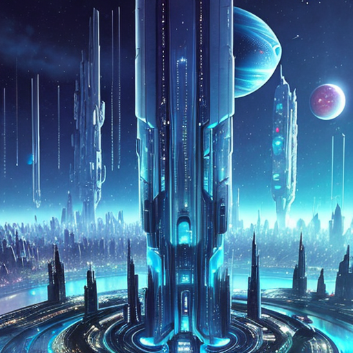

Image super-resolution
Another effective technique for fine-tuning a model is enhancing the resolution of the generated image. Unlike traditional image upscaling methods that rely on simple interpolation, image super-resolution leverages advanced algorithms, often powered by deep learning. These models learn high-frequency patterns and details from a dataset of high-resolution images, enabling them to produce superior-quality results when applied to low-resolution images.
Img2img diffusion
As previously discussed, Stable Diffusion models do not rely solely on text for initial guidance; they can also use an image as a starting point. The idea here involves leveraging the text-to-image pipeline to generate a small image (e.g., 256x256) and then applying an image-to-image model to upscale it, achieving a higher resolution.
# img2img pipeline
img2img_pipe = StableDiffusionImg2ImgPipeline.from_pretrained(
    "stablediffusionapi/deliberate-v2",
    torch_dtype = torch.float32,
    cache_dir = "/Volumes/ai-1t/diffuser"
).to("mps")

# upscale the image to 768 x 768
img2image_3x = img2img_pipe(
    prompt = prompt,
    negative_prompt = neg_prompt,
    image = resized_raw_image, # the original low-res image
    strength = 0.3,
    number_of_inference_steps = 80,
    guidance_scale = 8,
    generator = torch.Generator("mps").manual_seed(3)
).images[0]
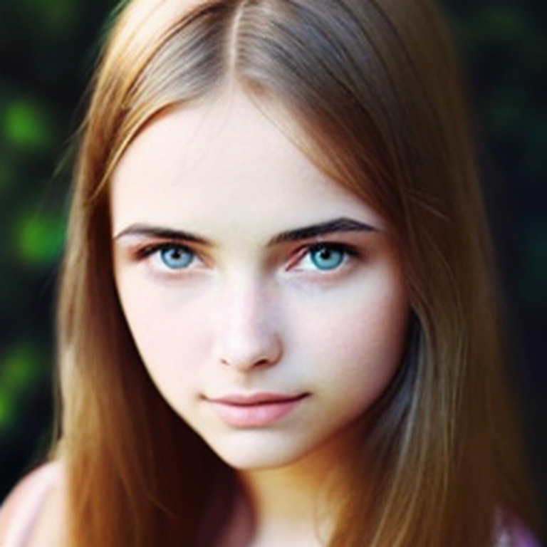
Below is a comparison between the raw image and the enhanced image. The model nearly enhanced every aspect of the image - from the eyebrows and eyelashes to the pupils and the mouth.

ControlNet
ControlNet is a neural network architecture designed to enhance diffusion models through the incorporation of additional conditions. It employs one or more supplementary UNet models that work alongside the Stable Diffusion model. These UNet models process both input prompt and the image concurrently, with results being merged back in each step of the UNet up-stage.
Compared with the img2img approach, ControlNet yields better outcomes. Among the ControlNet models, the ControlNet Tile stands out for its ability to upscale images by introducing substantial detail information to the original image.
# load the ControlNet model
controlnet = ControlNetModel.from_pretrained(
    "takuma104/control_v11",
    subfolder=  'control_v11f1e_sd15_tile',
    torch_dtype = torch.float32,
    cache_dir = "/Volumes/ai-1t/diffuser"
)

# upscale the image
cn_tile_upscale_img = pipeline(
    image = resized_raw_image,
    control_image = resized_raw_image,
    prompt = f"{sr_prompt}{prompt}",
    negative_prompt = neg_prompt,
    strength = 0.8,
    guidence_scale = 7,
    generator = torch.Generator("mps"),
    num_inference_steps = 50
).images[0]
Here we use the raw resized image to both the initial diffusion image and the ControlNet start image (control_image). The strength controls the influence of ControlNet on the denoising process.
Let’s use this prompt to compare the results between the generated raw image and the refined the image:
A stunningly realistic photo of a 25yo women with long, flowing brown hair and a beautiful smile.
upper body, detailed eyes, detailed face, realistic skin texture, set against a blue sky, with a few fluffy clouds in the background.
As you can see in the photos below, The ControlNet produces remarkable results
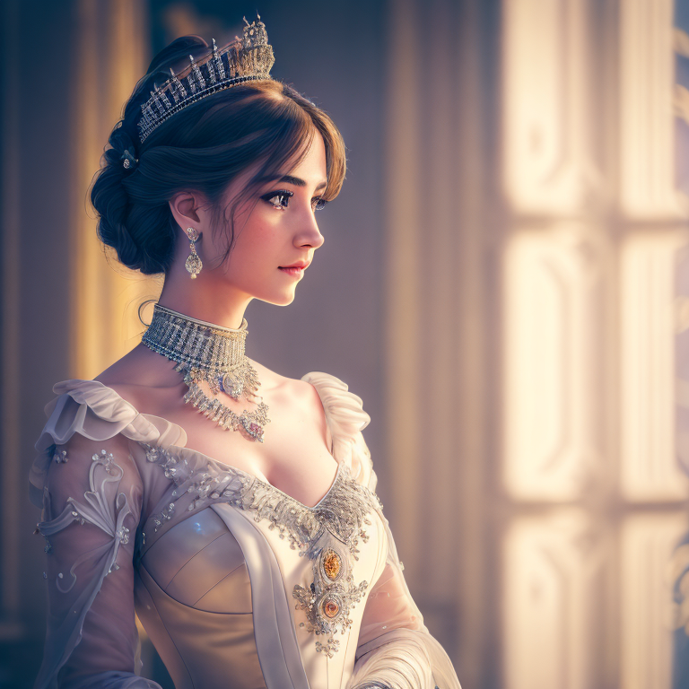
In the above example, the image-to-image approach would require multiple steps to achieve a desirable outcome. In contrast, the ControlNet Tile accomplish the same outcome with a single round of upscaling. Additionally, ControlNet Tile consumes relatively lower VRAM usage compared to the image-to-image solution.
If your goal is to preserve as many aspects of the original image as possible during the upscaling, the image-to-image approach would be a better option. Conversely, if you prefer an AI-driven, or a creative approach that generates new rich details, ControlNet Tile is a more preferable option.
More on ControlNet
It turns out that ControlNet is even more powerful than it initially appears. In addition to enhance the images at almost all aspects, it provides finer control for precise adjustments. For example, it is possible for ControlNet generate an image that replicates a specific pose from another image that the out-of-the-box Stable Diffusion model cannot achieve:
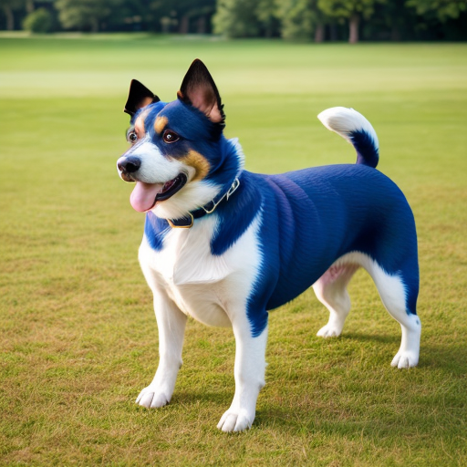
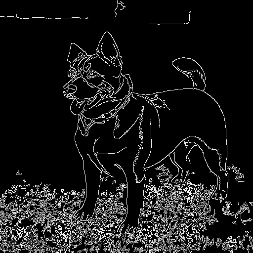
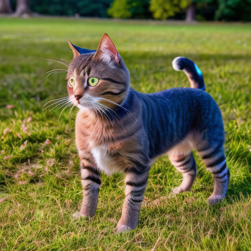
In the example above, we extracted edge information from the original photo and used it as a control image in the ControlNet pipeline. This allowed the generated image to replace the dog with a cat while preserving the dog’s original pose, thanks to the edge guidance.
Similarly, with the recent advancements in SDXL, we can extract pose information from a human body and transfer it to another person.
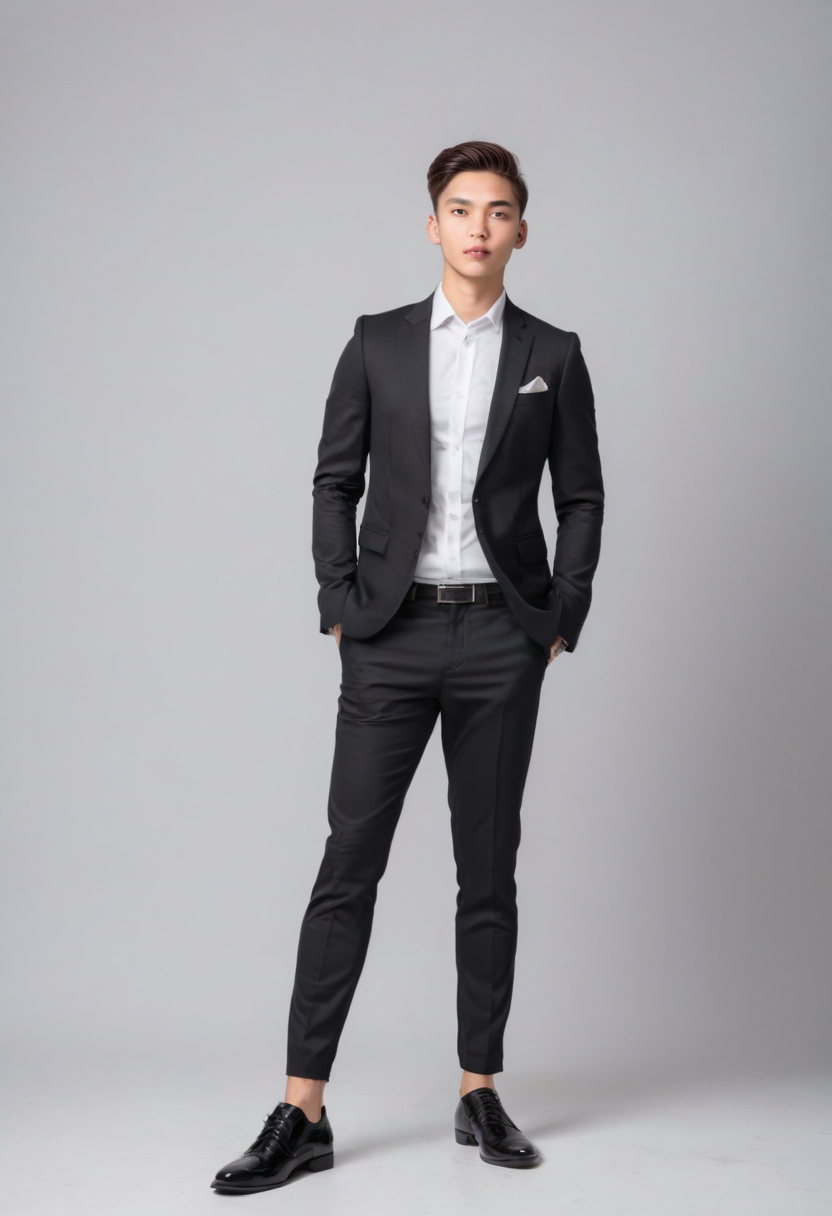
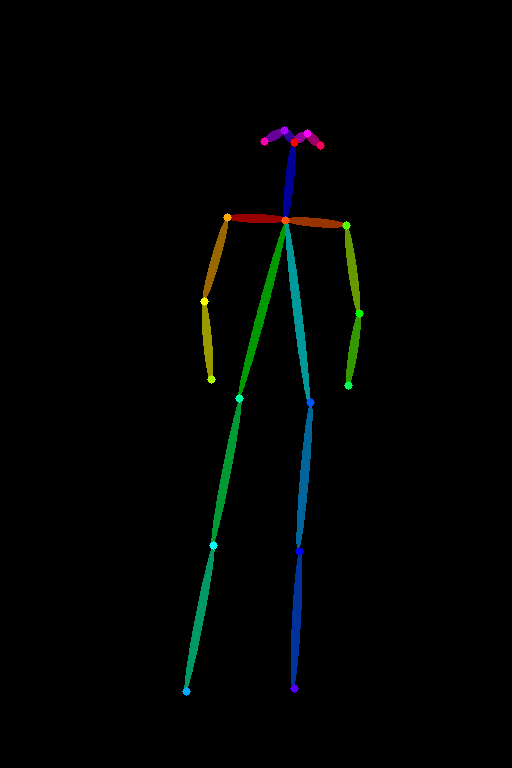
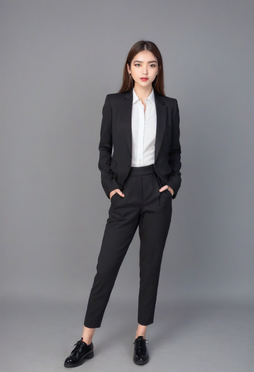
Note that the ControlNet models will only work with models using the same base model. A SD v1.5 ControlNet model works with all other SD v1.5 models. For SDXL models, we will need a ControlNet that is trained with SDXL. This is because SDXL models use a different architecture, a larger UNet than the SD v1.5.
How does ControlNet work
TBD
Summary
| Control Method | Functioning Stage | Usage Scenario |
|---|---|---|
| Textual Embedding | Text encoder | Add a new style, a new concept or a new face |
| LoRA | Merge LoRA weights to the UNet model (and the CLIP text encoder, optional) | Add a set of styles, concepts, and generate content |
| Image to Image | Provide the initial latent image | Fix images, or add styles and concepts to images |
| ControlNet | Participant denoising together with a checkpoint model UNet | Control shape, pose, content detail |