
LoRA Fine-Tuning
How LoRA Works
In previous articles, we briefly discussed LoRA as a method for fine-tuning LLMs. With LoRA, the original model remains unchanged and frozen, while the fine-tuned weight adjustments are stored separately in what is known as a LoRA file.
LoRA works by creating a small, low-rank model that is adapted for a specific concept. This small model can be merged with the main checkpoint model to generate images during the inference stage.
Let’s use $W$ to represent the original UNet attention weights(Q, K, V), $\Delta W$ to denote the fine-tuned weights from LoRA, and $W’$ as the combined weights. The process of adding LoRA to a model can be expressed as:
If we want to control the scale of LoRA weights, we can leverage a scale factor $\alpha$:
\[W' = W + \alpha\Delta W\]The range of $\alpha$ can be from 0 to 1.0. It should be fine if we set $\alpha$ slightly larger than 1.0.
The reason why LoRA is so small is that $\Delta W$ can be represented by two small low-rank matrices $A$ and $B$, such that:
\[\Delta W = AB^T\]Where $A$ is a n x d matrix, and $B$ is a m x d matrix. For example, if $\Delta W$ is a 6x8 matrix, there are a total of 48 weight numbers. Now, in the LoRA file, the 6x8 matrix can be decomposed into simply two small matrices — a 6x2 matrix (12 numbers in total) and another 2x8 matrix (16 numbers). The total trained parameters have been reduced from 48 to 28. This is why the LoRA file can be so small.
So, the overall idea of merging LoRA weights to the checkpoint model works like this:
- Find the $A$ and $B$ weight matrices from the LoRA file
- Match the LoRA module layer name to the model’s module layer name so that we know which matrix to patch
- Produce $\Delta W = AB^T$
- Update the model weights
The benefits of LoRA
-
Reduced resource consumption. Fine-tuning deep learning models typically requires substantial computational resources, which can be expensive and time-consuming. LoRA reduces the demand for resources while maintaining high performance.
-
Faster iterations. LoRA enables rapid iterations, making it easier to experiment with different fine-tuning tasks and adapt models quickly.
-
Improved transfer learning. LoRA enhances the effectiveness of transfer learning, as models with LoRA adapters can be fine-tuned with less data. This is particularly valuable in situations where labeled data is scarce.
LoRA in Practice
In this section, we will be using the CIFAR-10 dataset to train a basic image classifier from scratch using only several epochs. Following that, we further fine-tune the model with LoRA, illustrating the advantages of incorporating LoRA into the training process.
To recognize images in the dataset, we create a three layer classifier, focusing on simplicity to demonstrate how LoRA works.
class Classifier(nn.Module):
    def __init__(self):
        super().__init__()
        self.fc1 = nn.Linear(3*32*32, 4096)
        self.fc2 = nn.Linear(4096, 2048)
        self.fc3 = nn.Linear(2048, 10)

    def forward(self, x):
        x = torch.flatten(x, 1)
        x = F.relu(self.fc1(x))
        x = F.relu(self.fc2(x))
        x = fc3(x)
        return x
Next, we train the model for only 2 epochs and have a quick test. Given 8 random images in the dataset, the model predicts only 2 images correctly.
Ground truth labels:  cat  ship  ship     airplane  frog frog automobile frog
Predicted:            deer truck airplane ship      deer frog automobile bird
If we run the model on the test set over 10,000 images, the accuracy is about 32%. The result is somehow expected as the model is severely under-trained. Now, instead of training the same model with more epochs, we will freeze the model and apply LoRA to update the model’s weights.
class ParametrizationWithLoRA(nn.Module):
    def __init__(self, features_in, features_out, rank=4, alpha=1, device='cpu'):
        super().__init__()

        # Create A B and scale used in ∆W = BA x α/r
        self.lora_weights_A = nn.Parameter(torch.zeros((rank,features_out)).to(device))
        nn.init.normal_(self.lora_weights_A, mean=0, std=1)
        self.lora_weights_B = nn.Parameter(torch.zeros((features_in, rank)).to(device))

        # convert scale to device type
        # self.scale = torch.tensor(alpha / rank, dtype=torch.float32, device=device)
        self.scale = 1.0

    def forward(self, original_weights):
        return original_weights +
        torch.matmul(self.lora_weights_B, self.lora_weights_A).view(original_weights.shape) * self.scale


def apply_parameterization_lora(layer, device, rank=4, alpha=1):
        """
        Apply loRA to a given layer
        """
        features_in, features_out = layer.weight.shape
        return ParametrizationWithLoRA(
            features_in, features_out, rank=rank, alpha=alpha, device=device
        )

def apply_lora(model, device):
    parametrize.register_parametrization(model.fc1, "weight", apply_parameterization_lora(model.fc1, device))
    parametrize.register_parametrization(model.fc2, "weight", apply_parameterization_lora(model.fc2, device))
    parametrize.register_parametrization(model.fc3, "weight", apply_parameterization_lora(model.fc3, device))
To incorporate LoRA weights into the original model, we can leverage PyTorch’s parameterization mechanism. The key idea is to augment each linear layer by updating its weights using LoRA’s low-rank matrices: lora_weights_A and lora_weights_B.
As a result, the model’s parameters now consist of two components: the original weights and the additional parameters introduced by LoRA:
fc1:  fc1.parametrizations.weight.original
fc1:  fc1.parametrizations.weight.0.lora_weights_A
fc1:  fc1.parametrizations.weight.0.lora_weights_B
In this setup, we set the LoRA rank to 4, which results in lora_weights_A having shape [4, N] and lora_weights_B having shape [M, 4].
Before training the LoRA, let’s examine the additional parameters introduced by LoRA:
Number of parameters in the original model: 20,998,154
Parameters added by LoRA: 15,370
Parameters increment: 0.073%
The LoRA only adds 0.073% parameters to our model.
To re-train the model with LoRA, we need to freeze all the model’s original parameters:
for name, param in model.named_parameters():
    if 'lora' not in name:
        param.requires_grad = False
The training process for LoRA follows the same procedure as the original model. Let’s train it for 2 epochs and observe its performance. We’ll evaluate the results using the same set of 8 test images:
Ground truth labels:  cat ship ship airplane frog frog automobile frog
Predicted:            cat ship ship ship     deer frog dog        deer
The model correctly classifies 4 out of 8 images. When evaluated on the full test set, it achieves 42% accuracy(previously 32%), indicating that the parameters have learned meaningful representations.
LoRA in Stable Diffusion
To train LoRA for Stable Diffusion models, we can leverage the LoRAConfig features from HuggingFace’s PEFT library:
unet_lora_config = LoraConfig(
    r                   = lora_rank,
    lora_alpha          = lora_alpha,
    init_lora_weights   = "gaussian",
    target_modules      = ["to_k", "to_q", "to_v", "to_out.0"]
)
unet.add_adapter(unet_lora_config)
The core idea is to update the attention weights within the Transformer blocks to better guide noise prediction in the U-Net.
To utilize LoRA, we can leverage the load_lora_weights function from the StableDiffusionPipeline class.
pipe.load_lora_weights(
    pretrained_model_name_or_path_or_dict=lora_model_path,
    adapter_name="az_lora"
)
pipe.set_adapters(["az_lora"], adapter_weights=[1.0])
In the following example, we use 100 Van Gogh-style images to train a LoRA model. Each image is paired with the same descriptive caption, as shown below:
{"file_name": "001.png", "text": "a painting in vangogh style"}
{"file_name": "002.png", "text": "a painting in vangogh style"}
...
The trained LoRA model takes only 2.3MB compared to the base sd-1.5 model. To test our LoRA, we generate an image using the following prompt:
prompt = "a dog sitting on a beach. a painting in vangogh style"
Note that the prompt has to contain the text used to train our LoRA. Below, we compare the results before and after LoRA fine-tuning:
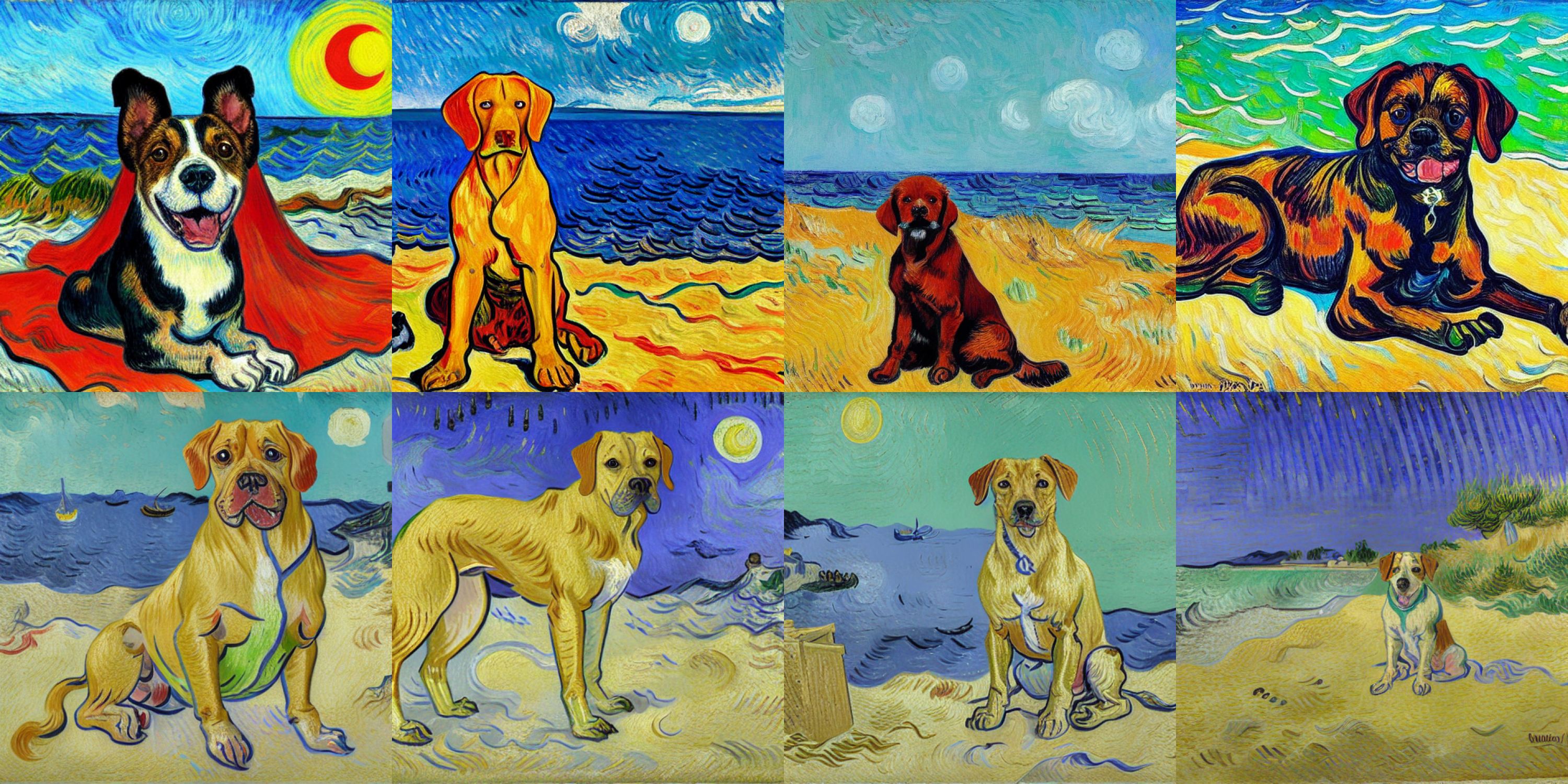
The first row shows images generated by the original Stable Diffusion 1.5 model. The second row shows results after fine-tuning with our Van Gogh-style LoRA model.