The Transformer Architecture
Generative models before Transformer
Previous generations of language models made use of an architecture called RNN. RNNs while powerful for their time, were limited by the amount of compute and memory needed to perform well at generative tasks.
To successfully predict the next word, models need to see more than just the previous few words. Models needs to have an understanding of the whole sentence or even the whole document.
Attention is all you need
In 2017, after the publication of this paper, “Attention is All You Need”, from Google and the University of Toronto. The transformer architecture had arrived. This novel approach unlocked the progress in generative AI that we see today. It can be scaled efficiently to use multi-core GPUs, it can parallel process input data, making use of much larger training datasets, and crucially, it’s able to learn to pay attention to the meaning of the words it’s processing.
The power of the attention mechanism lies in its ability to learn the relevance and context of all of the words in a sentence, not just the words next to its neighbors, but every other word in a sentence.

We apply attention weights to those relationships so that the model learns the relevance of each word to each other words no matter where they are in the input. This gives the algorithm the ability to learn “who has the book”, “who could have the book”, and if it’s even relevant to the wider context of the document.
These attention weights are learned during LLM training. In the end, we will learn something called “attention map”, which can be useful to illustrate the attention weights between each word and every other words.
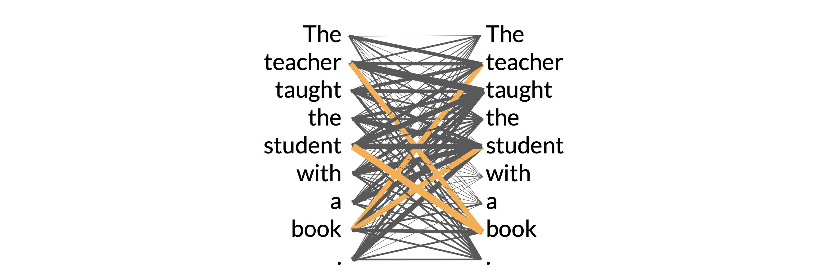
In this example, you can see that the word book is strongly connected with the word teacher and the word student.
This is called self-attention and the ability to learn attention in this way across the whole input significantly improves the model’s ability to encode language
The Transformer Architecture Overview
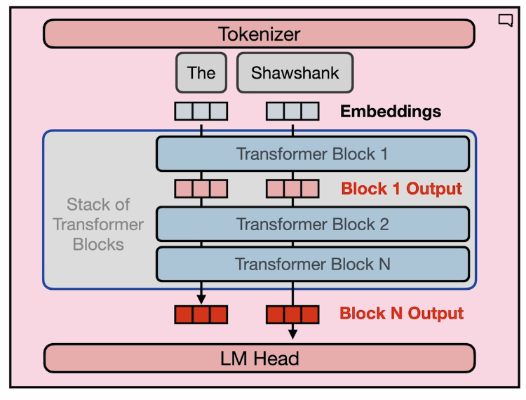
Tokenizer
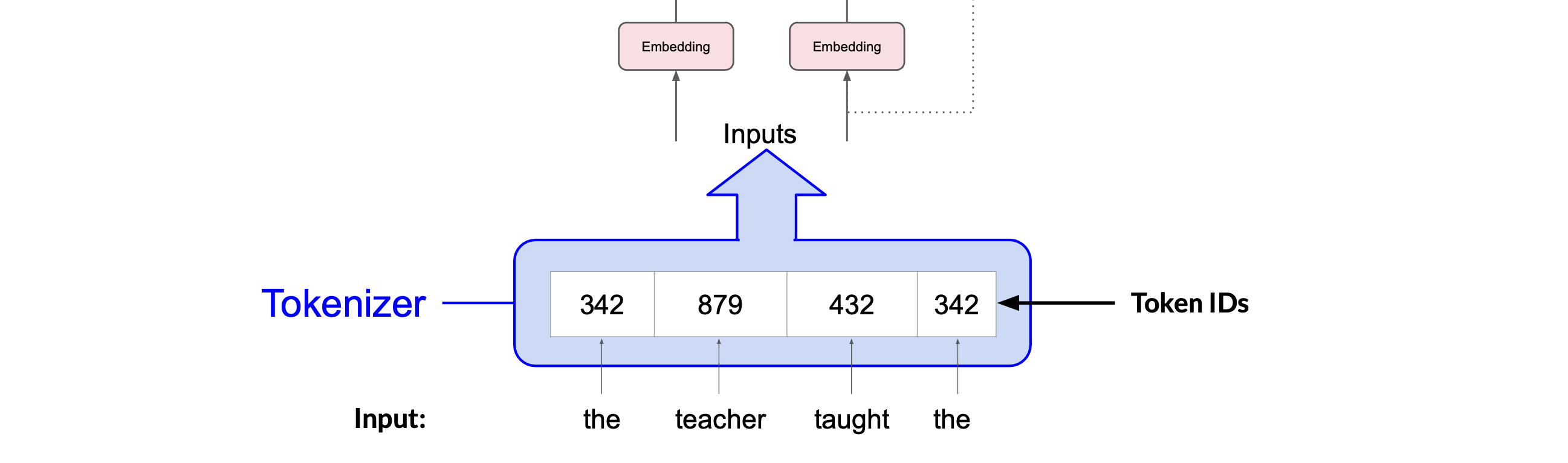
The inputs are first converted to tokens(one-hot vectors), with each number representing a position in a dictionary of all the possible words that the model can work with.
What’s important is that once you’ve selected a tokenizer to train the model, you must use the same tokenizer when you generate text. For example,
sentence = "Hello world!"

# load the pretrained tokenizer
tokenizer = AutoTokenizer.from_pretrained("bert-base-cased")

# apply the tokenizer to the sentence and extract the token ids
token_ids = tokenizer(sentence).input_ids

print(token_ids) #[101, 8667, 1362, 106, 102]
Embedding
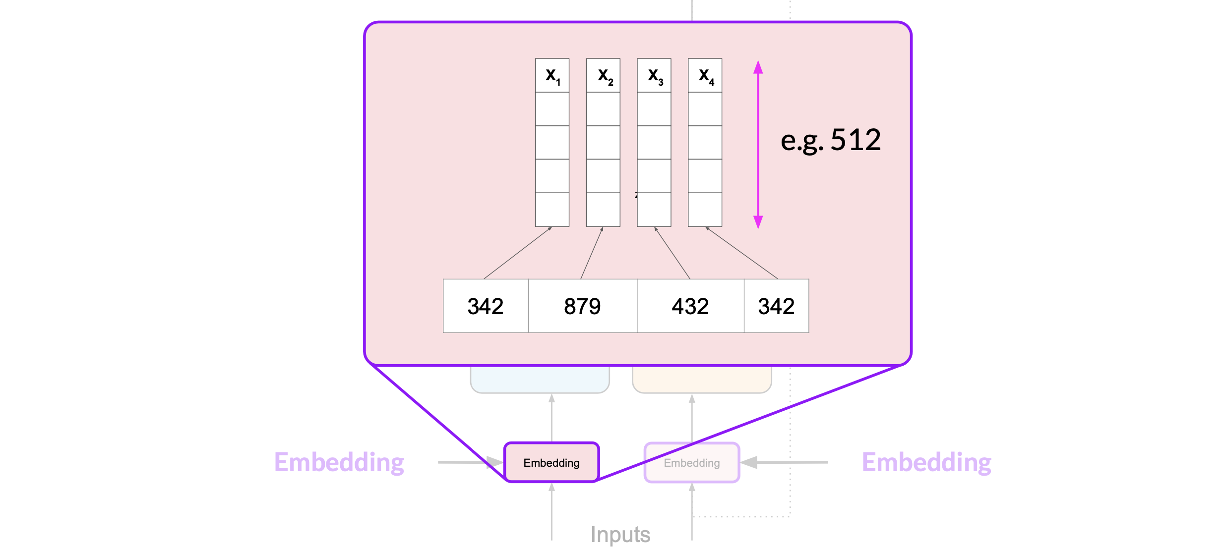
Now that your input is represented as numbers, you can pass it to the embedding layer. This layer is a trainable vector embedding space, a high-dimensional space where each token is represented as a vector and occupies a unique location within that space. The intuition is that these vectors learn to encode the meaning and context of individual tokens in the input sequence
In the original transformer paper, the vector size was actually 512.
For simplicity, if you imagine a vector size of just three, you could plot the words into a three-dimensional space and see the relationships between those words and calculate the distance between those words.
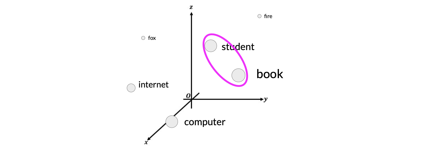
For example, the word “student” and “book” has closer relationship than “student” and “fire”. In the embedding space, this means these two vectors are closer and have higher cosine similarities.
More detail about word embeddings can be found in the previous post
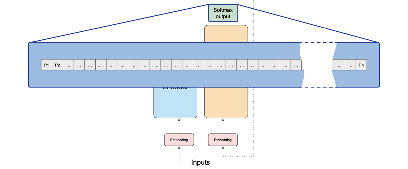
Positional Encoding
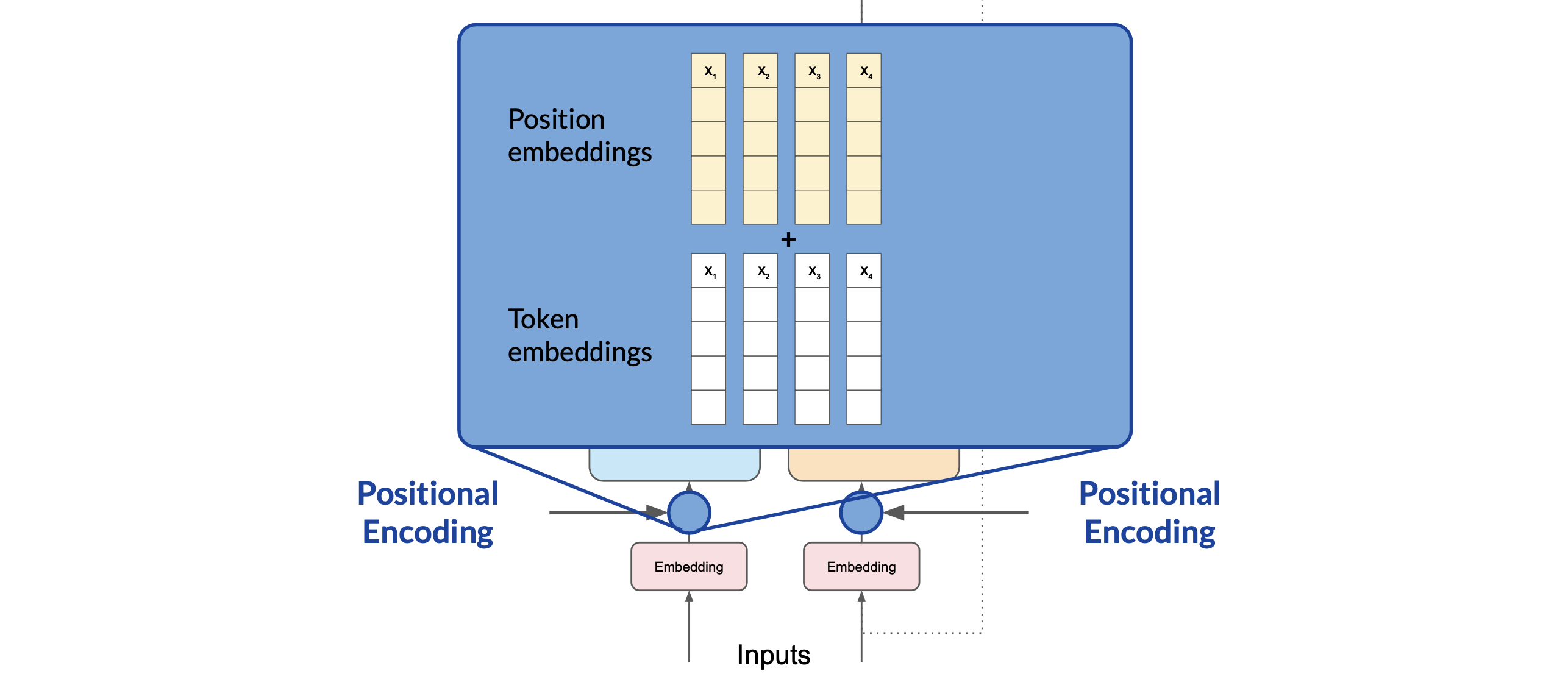
Since the model processes each of the input tokens in parallel. We need to preserve the information about the word order and don’t lose the relevance of the position of the word in the sentence. We do so by adding the positional encoding. Once the positional encoding vectors are merged into the input tokens, we pass the resulting vectors to the self-attention layer.
The model analyzes the relationships between the tokens in your input sequence. This allows the model to attend to different parts of the input sequence to better capture the contextual dependencies between the words.
The transformer block
The self-attention weights that are learned during training and stored in these layers reflect the importance of each word in that input sequence to all other words in the sequence. But this does not happen just once, the transformer architecture actually has multi-headed self-attention.
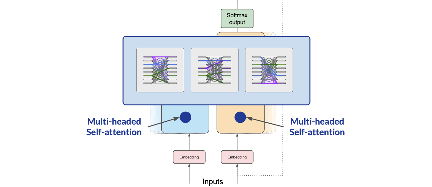
This means that multiple sets of self-attention weights or heads are learned in parallel independently of each other. The number of attention heads included in the attention layer varies from model to model, but numbers in the range of 12 to 100 are common.
The intuition here is that each self-attention head will learn a different aspect of language. For example, one head may see the relationship between the people entities in our sentence. While another head may focus on the activity of the sentence.
It is important to note that we don't dictate ahead of time what aspects of language the attention heads will learn. The weights of each head are randomly initialized and given sufficient training data and time, each will learn different aspects of language.
We’ll discuss more about the self-attention mechanism in great detail in the next post
LM Head
Now the output is processed through a fully-connected feed-forward network followed by a softmax layer. The output of this layer is a vector of logits proportional to the probability score for each and every token in the tokenizer dictionary. You can then pass these logits to a final softmax layer, where they are normalized into a probability score for each word
The outputs are normalized into a probability score for each word. This output includes a probability for every single word in the dictionary, so there’s likely to be thousands of scores here.
The word generation process
Once we have the generated word, we simply append it back to the original sentence, and use it for the next word generation. The whole generation process is a loop:
for i in range(max_new_tokens):
    # Forward pass
    logits = model(input_ids=generated_ids, attention_mask=torch.ones_like(generated_ids))
    # torch.Size([1, 6, 32000])
    # (batch, The sequence length of the input, vocab size)

    # Get the last token's logits
    next_token_logits = logits[:, -1, :]
    # Greedy decoding: pick the token with the highest probability
    next_token_id = next_token_logits.argmax(dim=-1).unsqueeze(0)
    # Decode the token ID to string
    next_token_str = tokenizer.decode(next_token_id[0].item())
    # Append next token to the generated_ids
    generated_ids = torch.cat([generated_ids, next_token_id], dim=1)
    # Decode the entire sequence back into text
    output_text = tokenizer.decode(generated_ids[0], skip_special_tokens=True)
    # If the model has an EOS token and we encounter it, break
    if next_token_id.item() == tokenizer.eos_token_id:
        break
Model Example
To piece everything together, we will be using the Microsoft’s Phi-3-mini-4k-instruct
# get the model
model = AutoModelForCausalLM.from_pretrained(
    "microsoft/Phi-3-mini-4k-instruct",
    cache_dir=cache_dir,
    device_map="cpu",
    torch_dtype="auto",
    trust_remote_code=True,
)
The Phi-3-mini-4k-instruct model architecture
Let’s print out the model structure:
Phi3ForCausalLM(
  (model): Phi3Model(
    (embed_tokens): Embedding(32064, 3072, padding_idx=32000)
    (embed_dropout): Dropout(p=0.0, inplace=False)
    (layers): ModuleList(
      (0-31): 32 x Phi3DecoderLayer(
        (self_attn): Phi3Attention(
          (o_proj): Linear(in_features=3072, out_features=3072, bias=False)
          (qkv_proj): Linear(in_features=3072, out_features=9216, bias=False)
          (rotary_emb): Phi3RotaryEmbedding()
        )
        (mlp): Phi3MLP(
          (gate_up_proj): Linear(in_features=3072, out_features=16384, bias=False)
          (down_proj): Linear(in_features=8192, out_features=3072, bias=False)
          (activation_fn): SiLU()
        )
        (input_layernorm): Phi3RMSNorm()
        (resid_attn_dropout): Dropout(p=0.0, inplace=False)
        (resid_mlp_dropout): Dropout(p=0.0, inplace=False)
        (post_attention_layernorm): Phi3RMSNorm()
      )
    )
    (norm): Phi3RMSNorm()
  )
  (lm_head): Linear(in_features=3072, out_features=32064, bias=False)
)
Embedding(32064, 3072, padding_idx=32000)
Phi3DecoderLayer(
  (self_attn): Phi3Attention(
    (o_proj): Linear(in_features=3072, out_features=3072, bias=False)
    (qkv_proj): Linear(in_features=3072, out_features=9216, bias=False)
    (rotary_emb): Phi3RotaryEmbedding()
  )
  (mlp): Phi3MLP(
    (gate_up_proj): Linear(in_features=3072, out_features=16384, bias=False)
    (down_proj): Linear(in_features=8192, out_features=3072, bias=False)
    (activation_fn): SiLU()
  )
  (input_layernorm): Phi3RMSNorm()
  (resid_attn_dropout): Dropout(p=0.0, inplace=False)
  (resid_mlp_dropout): Dropout(p=0.0, inplace=False)
  (post_attention_layernorm): Phi3RMSNorm()
)
The model has two main components - model and lm_head.
- The
modelconsists an embedding layer and 32 transformer blocks.- The embedding vector size is
(32064, 3072), meaning the vocabulary size is32064and each embedding vector has3072dimensions - There are 32 transformer layers(blocks).
- The self attention module (
self_atten) has three parts:o_projthe output of the attention head. It is a linear layer. The goal is to project the attention output back to the original hidden size (3072 in this case).rotary_embis the positional encoding moduleqkv_projis the self-attention ahead- The
9216output is then split into 3 equal parts:- Q: shape (batch_size, seq_len,
3072) - K: shape (batch_size, seq_len,
3072) - V: shape (batch_size, seq_len,
3072)
- Q: shape (batch_size, seq_len,
- These three matrices are generated from the same `qkv_proj` linear layer by slicing the output tensor.
- The
- The mlp module contains two linear layers and an activation function
gate_up_projlayer outputs two tensors, by splitting the16384output into two8192parts:- One part goes through a non-linearity (like
SiLU) - The other part is used as a gating mechanism (element-wise multiplication)
hidden = gate_up_proj(x) # shape: [batch, seq_len, 16384] a, b = hidden.chunk(2, dim=-1) # each: [batch, seq_len, 8192] gated = SiLU(a) * b # shape: [batch, seq_len, 8192] output = down_proj(gated) # shape: [batch, seq_len, 3072]- One part goes through a non-linearity (like
- The self attention module (
- The embedding vector size is
- The
lm_headis just a linear layer that maps the3072dimensional vectors and output the probability of the next word among32064words.
Examine individual components
We could also inspect the individual components of the model using a test prompt. Let’s say we have a five-word text prompt shown as below, and we expect the predicted word to be Pairs:
prompt = "The capital of France is"
Let analyze the model’s components step by step:
- Check the input’s token_ids:
input_ids = tokenizer(prompt, return_tensors="pt").input_ids
print("tokens: ", input_ids) # tensor([[ 450, 7483,  310, 3444,  338]])
- Check the input’s embeddings:
# get the embedding model
em = model.model.embed_tokens(input_ids)
print("embeddings: ", em(input_ids).shape) # torch.Size([1, 5, 3072])
- Check the output of the first attention head in the transformer block:
att1 = model.model.layers[0].self_attn.o_proj(embeddings)
print("att1: ", att1.shape) # torch.Size([1, 5, 3072])
- Check the output of the transformer block:
model_output = model.model(input_ids).last_hidden_state
print(model_output.shape)  # torch.Size([1, 5, 3072])
- Check the output of the last layer
lm_head:
lm_head_output = model.lm_head(model_output)
print("lm_head: ", lm_head_output.shape) # torch.Size([1, 5, 32064])
- Decode the predicted token to text:
token_id = lm_head_output[0,-1].argmax(-1)
print(token_id) # tensor(3681)
print(tokenizer.decode(token_id)) # Paris
Resources
- Generative AI with Large Language Models
- How Transformer LLMs work
- Attention is All You Need
- Vector Space Models
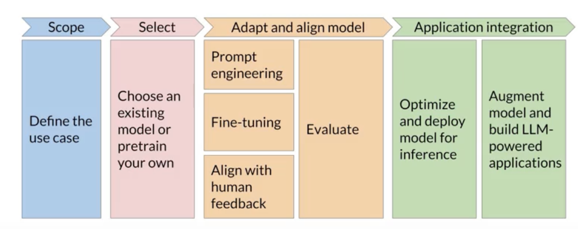
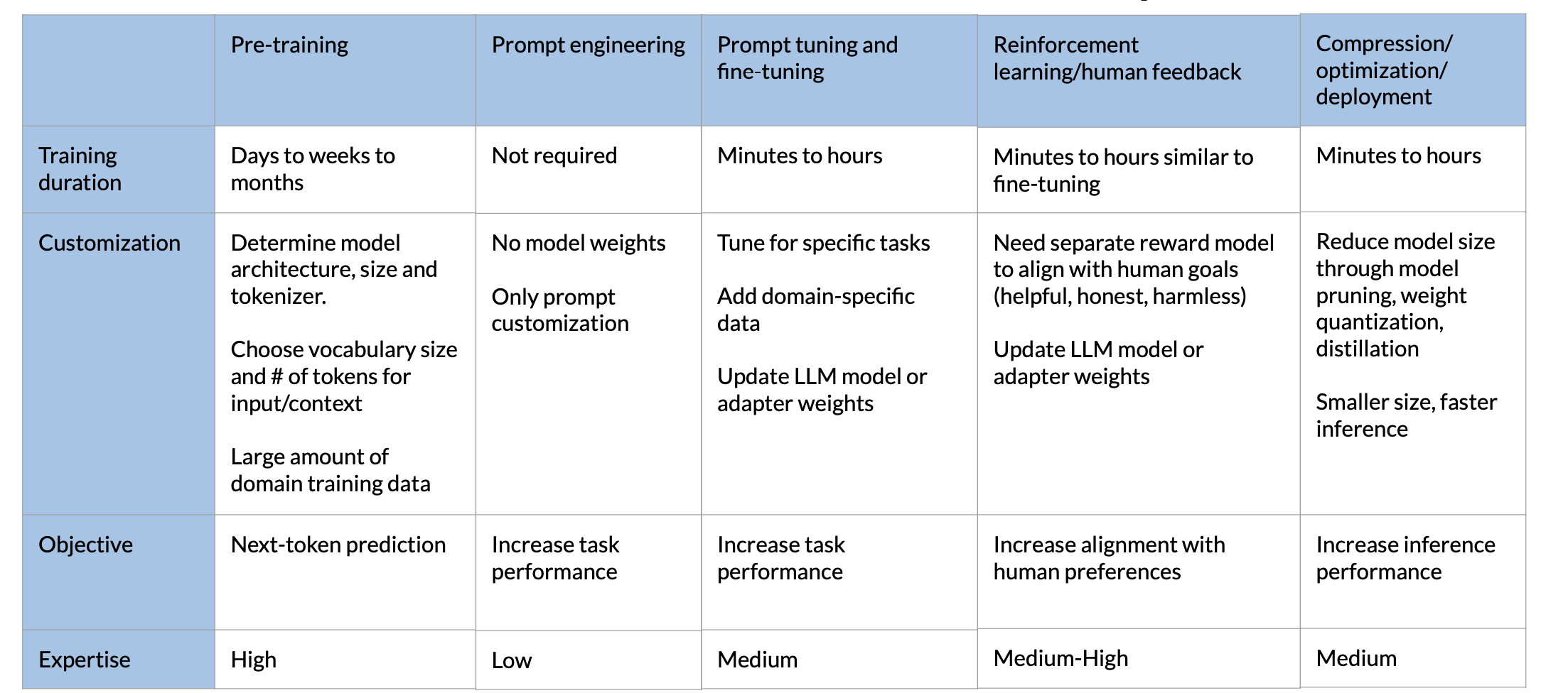
Appendix #1: GenAI project lifecycle